Cyclostationary Analysis of Lattice-Based Modulation

Introduction

Lattice Types

Lattices have been considered for use in digital communications, coding theory, cryptography, and have broad applications in geometry and physics, where their dense structure enables efficient representation and processing of multidimensional data [1-5].

The main draw towards using lattice based modulation in digital communications is to target up to 1.53 dB of shaping gain over traditional Quadrature-Amplitude Modulation (QAM) schemes [6]. While QAMs rotated across large N-dimensional spaces [cite UBDM] can create the illusion of Gaussianity in 1D/2D projections due to the Central Limit Theorem, the joint N-dimensional probability density function remains strictly uniform inside a rotated box. Real shaping gain requires pruning high-energy corner points of the N-box, which a pure rotation cannot perform. Lattice Voronoi cells (the set of all points in ℝ^n closest to a specific lattice point) provide a structured method of pruning these high-energy corners, with lattice voronoi cells approaching N-spheres rather than N-boxes.

A lattice of dimension n is a discrete set of points in Euclidean space generated by all integer linear combinations of a set of linearly independent basis vectors. Λ = {Bz : z ∈ ℤⁿ} where B is an n x n basis matrix defining the mapping between ℤⁿ and Λ. There may exist many different basis matrices that produce identical lattices, the only differences being the integer vector “labelings” of the lattice points.

The simplest lattice is the Z1 lattice consisting of all integers on the real number line: Z1 = {x ∈ ℤ}. The next simplest lattice is the Z2 lattice, which is the rectangular grid: Z2 = {(x₁, x₂) ∈ ℤ²}. Notice that since both dimensions of the Z2 lattice are independent of the other, in practice it is often easier to treat the Z2 lattice as two independent sets of Z1 lattices.

Rampart also considers the A2, D4, and E8 lattices. These provide the densest sphere packings in two, four, and eight dimensions, respectively [6]. Lattices are standardly named via a letter and a number. The letter corresponds to a generalized method of constructing lattices of the same family, while the number corresponds to the number of dimensions of the lattice.

The A2 lattice defined as A2 = {(x₁, x₂, x₃) ∈ ℤ³ : x₁ + x₂ + x₃ = 0} forms a two-dimensional lattice embedded in ℝ³, and is commonly referred to as the “hexagonal lattice”. On a 2D plane, this lattice consists of the set of points formed by the vertices of equilateral triangles tessellated to fill the entire plane, creating hexagonal Voronoi cells.

The D4 lattice defined as D4 = {x ∈ ℤ⁴ : x₁ + x₂ + x₃ + x₄ ≡ 0 (mod 2)} is commonly referred to as the “checkerboard lattice.” This is due to the fact that D4 is the 4-dimensional generalization of the D2 lattice, which resembles a checkerboard, picking every other point of the Z2 lattice.

The E8 lattice defined by E8 = D8 ∪ (D8 + (1/2)(1,1,1,1,1,1,1,1)), where D8 = {x ∈ ℤ⁸ : x₁ + x₂ + ··· + x₈ ≡ 0 (mod 2)} is composed of two cosets of the D8 lattice. This is the highest dimensional lattice considered in this cyclostationary evaluation.

Infinite lattices are not of practical use in digital communications. Instead, we work with a well-defined subset of the lattice, shaped by the lattice’s fundamental Voronoi cell. We define a modulus variable r, restricting the number of integer options per dimension (i.e. z_n ∈ {0, 1, 2, …, r}), and bits per lattice point as Log2(r)*n. See that when paired with a modulus, the Z2(r) lattice represents familiar QAMs. Z2(2)=QPSK, Z2(4) = 16QAM, Z2(8) = 64 QAM, and so on.

As mentioned earlier, Z2 lattices can be treated as two independent sets of Z1 lattices, similar to how QPSK constellations can derive bit LLR values for I and Q independently from a given IQ symbol. For the rest of this document, when we refer to Z1 lattices and unless otherwise specified, it should be assumed that we are actually referring to Z2 lattices in order to supply both In-phase and Quadrature values for IQ symbols (e.g. Z1(2) = Z2(2) = QPSK). When we wish to talk about actual Z1 lattices transmitted over a channel, such as a BPSK signal (the TRUE Z1(2) lattice), we explicitly mark it as either BPSK or a pulse-amplitude modulated (PAM) signal.

Additional definitions, properties, and constructions of these lattices can be found in [6].

Citations

1. S. Li, A. Mirani, M. Karlsson and E. Agrell, “Low-Complexity Voronoi Shaping for the Gaussian Channel,” in IEEE Transactions on Communications, vol. 70, no. 2, pp. 865-873, Feb. 2022, doi: 10.1109/TCOMM.2021.3130286.
2. Li, S., Mirani, A., Karlsson, M. et al (2021). Designing Voronoi Constellations to Minimize Bit Error Rate. IEEE International Symposium on Information Theory – Proceedings, 2021-July: 1017-1022. http://dx.doi.org/10.1109/ISIT45174.2021.9517815
3. M. Sadeghi, “Design and Analysis of Lattice-Based Communication Schemes: A Study of Constructions A and D,” Ph.D. dissertation, School of Eng., University of British Columbia, Kelowna, BC, Canada, 2025.
4. J. Conway and N. Sloane, “A fast encoding method for lattice codes and quantizers,” in IEEE Transactions on Information Theory, vol. 29, no. 6, pp. 820-824, November 1983, doi: 10.1109/TIT.1983.1056761.
5. B. M. Kurkoski, “Encoding and Indexing of Lattice Codes,” in IEEE Transactions on Information Theory, vol. 64, no. 9, pp. 6320-6332, Sept. 2018, doi: 10.1109/TIT.2018.2839181.
6. J. H. Conway and N. J. A. Sloane, Sphere Packings, Lattices and Groups, 3rd ed. New York: Springer, 1999, doi: org/10.1007/978-1-4757-6568-7.
7. B. M. Kurkoski, “The E8 lattice and error correction in multi-level flash memory,” in Proc. IEEE Int. Conf. Commun. (ICC), Kyoto, Japan, Jun. 2011, pp. 1-5.
8. J. Xue and B. M. Kurkoski, “Finite Dimensional Lattice Codes With Self Error-Detection and Retry Decoding,” in IEEE Transactions on Communications, vol. 73, no. 10, pp. 8484-8499, Oct. 2025, doi: 10.1109/TCOMM.2025.3560348.

Cyclostationary Plots

The two main cyclostationary plots discussed here are the Cyclic Autocorrelation Function, or CAF, and the Spectral Correlation Function, SCF. Descriptions of each function can be found in detail through Spooner’s work [9]. As well, there are two main pulse shape filters used in the following plots: the boxcar filter and the root raised cosine (RRC) filter, which uses a beta value of 0.35 or 0.8.

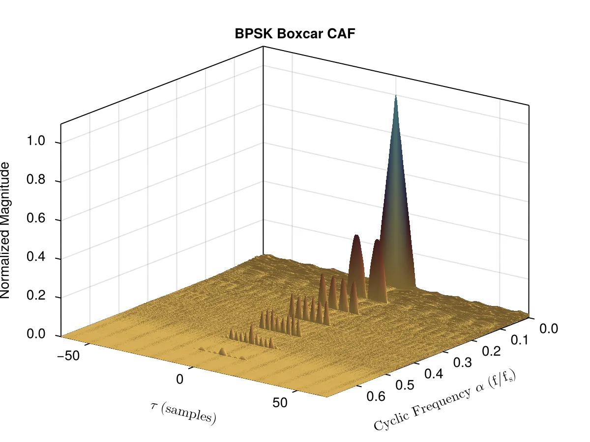
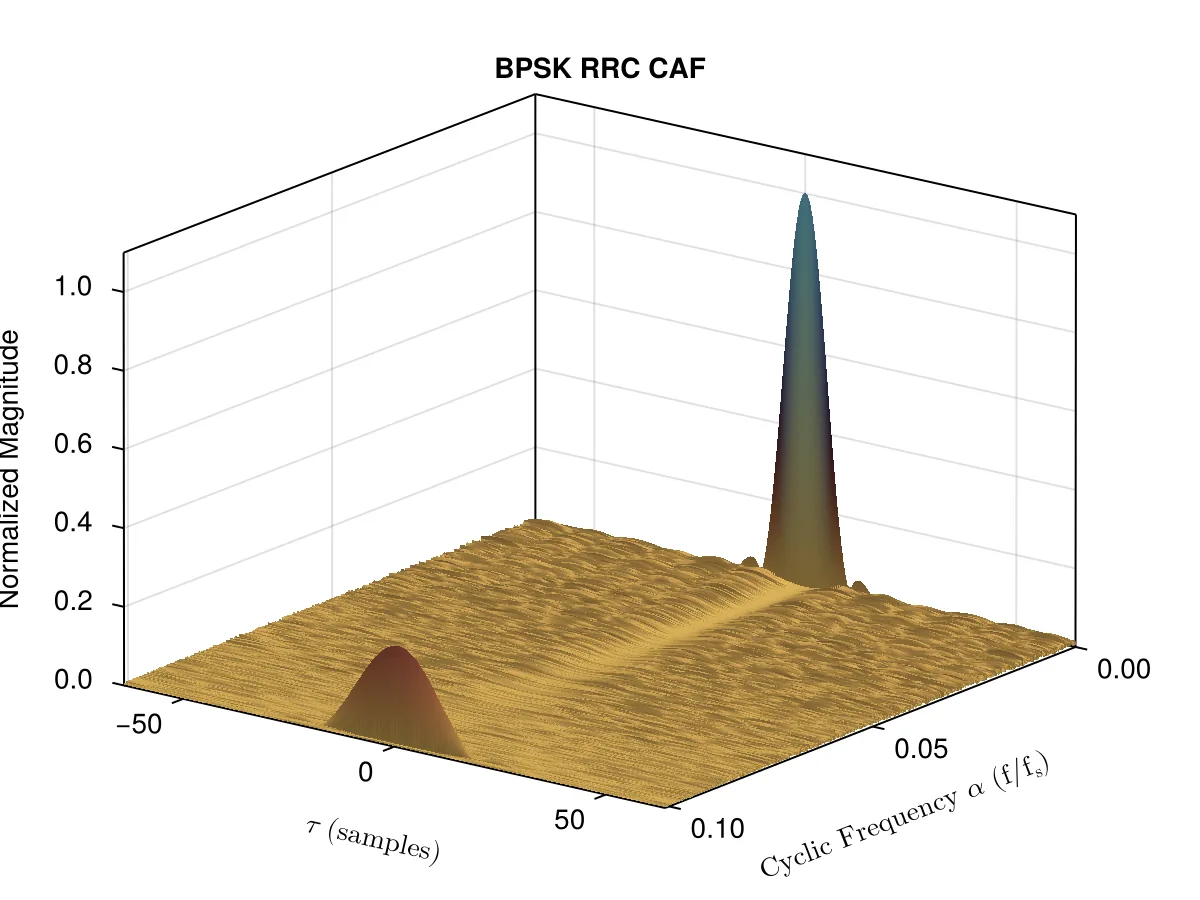
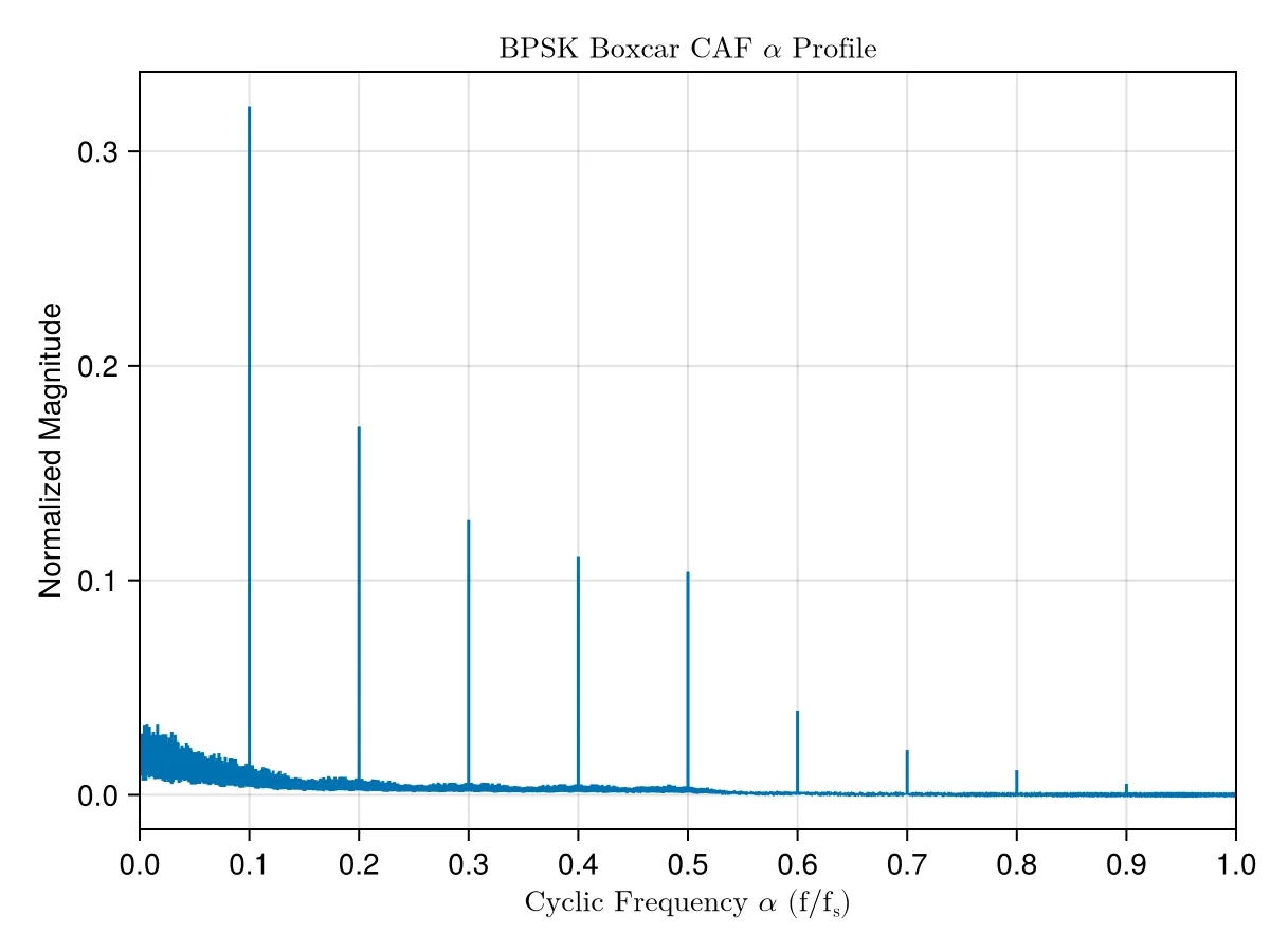
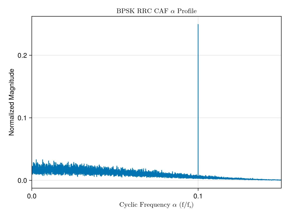
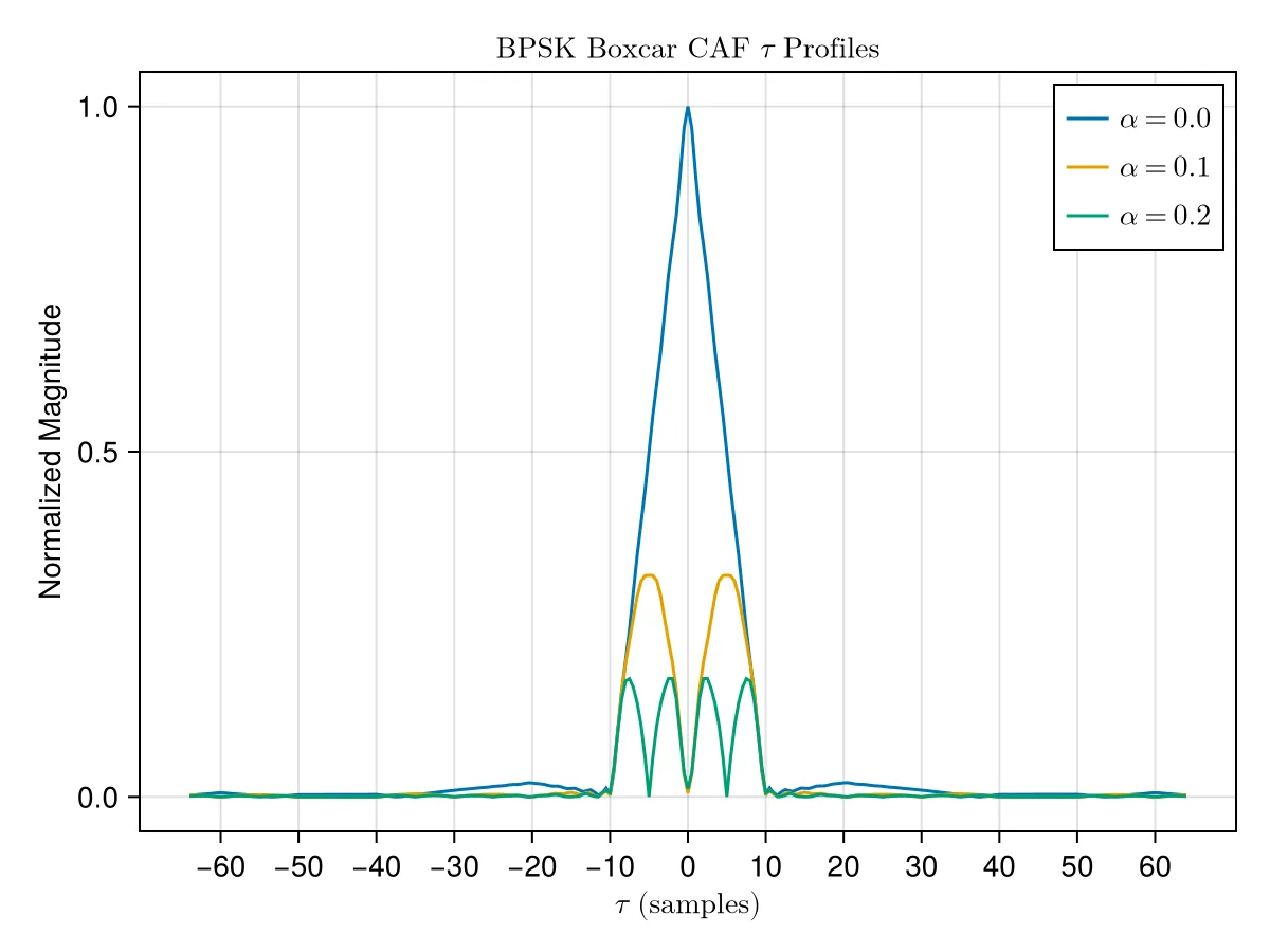
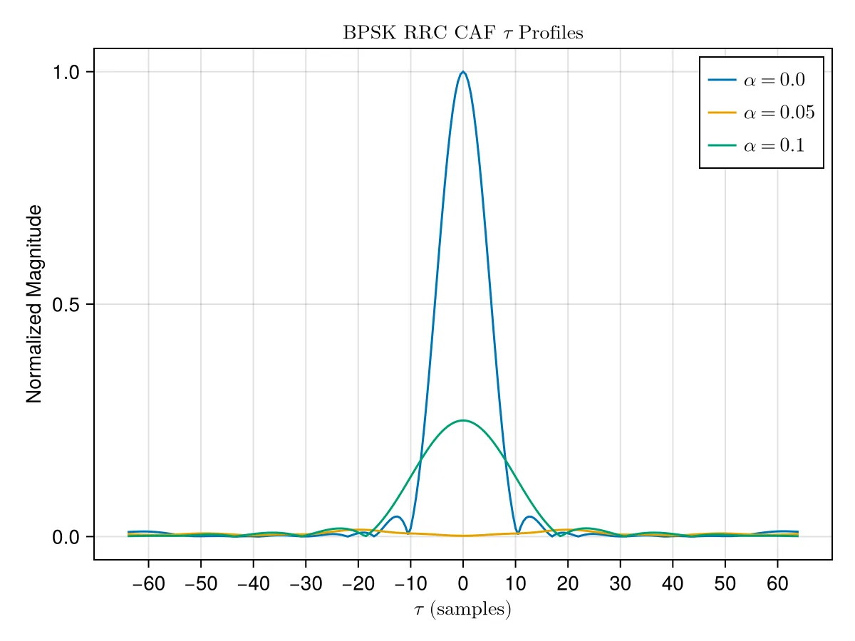
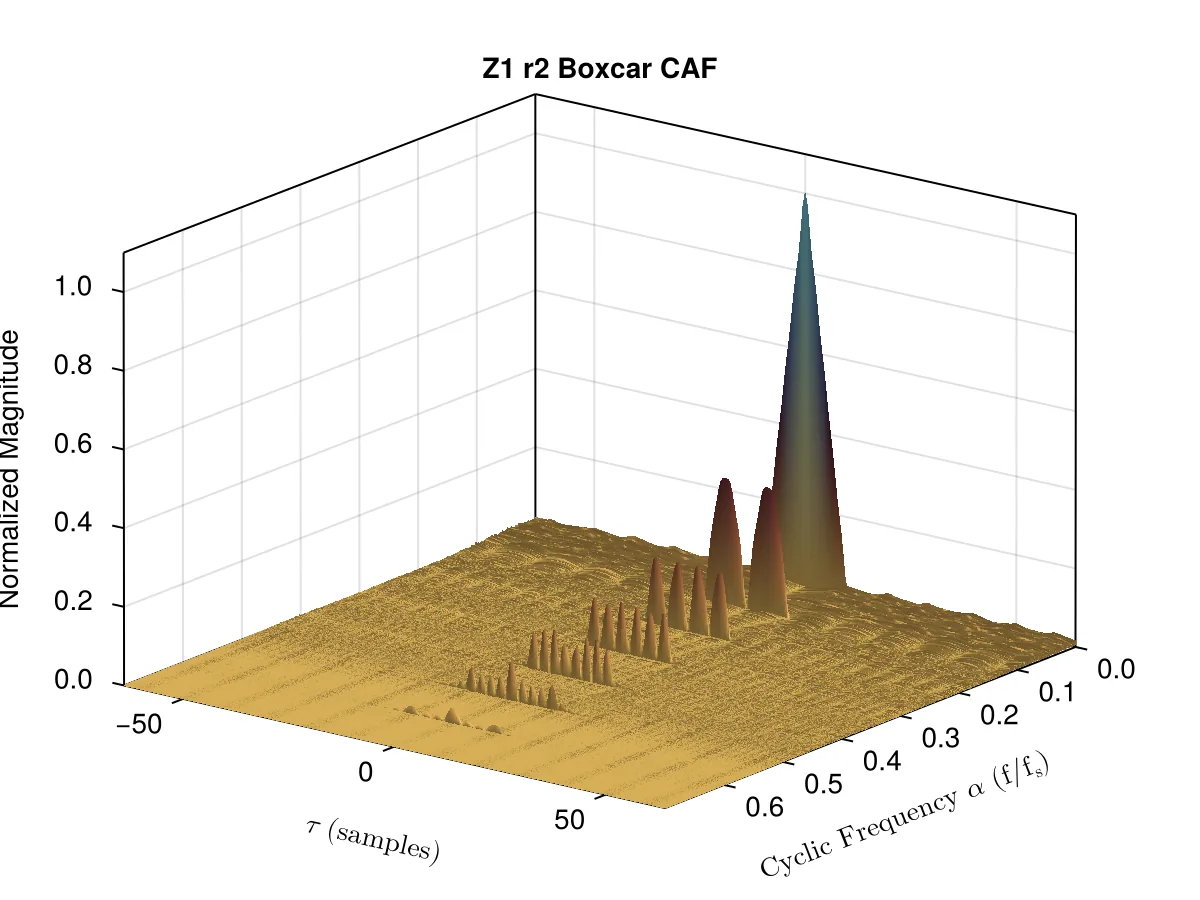
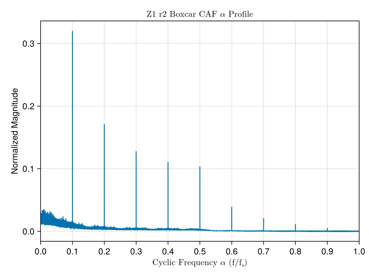
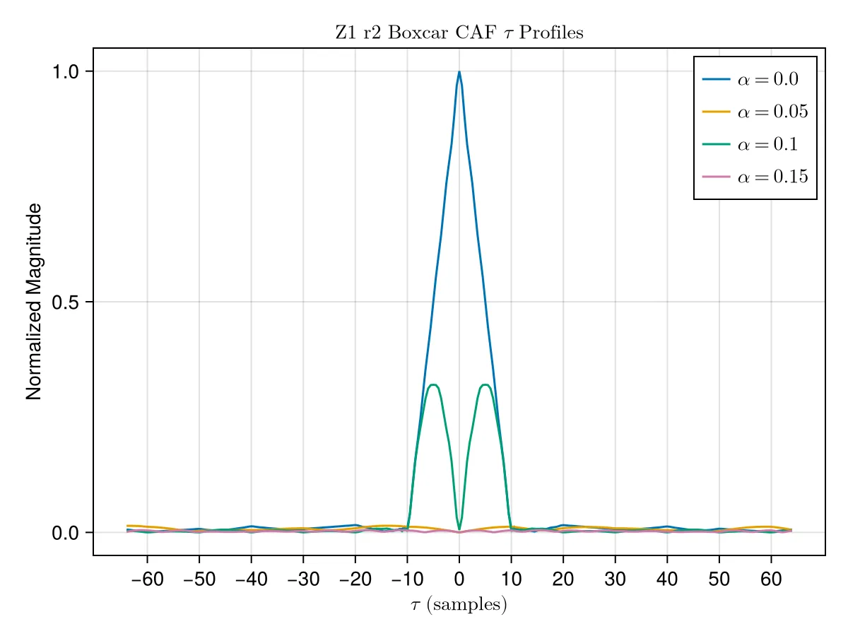
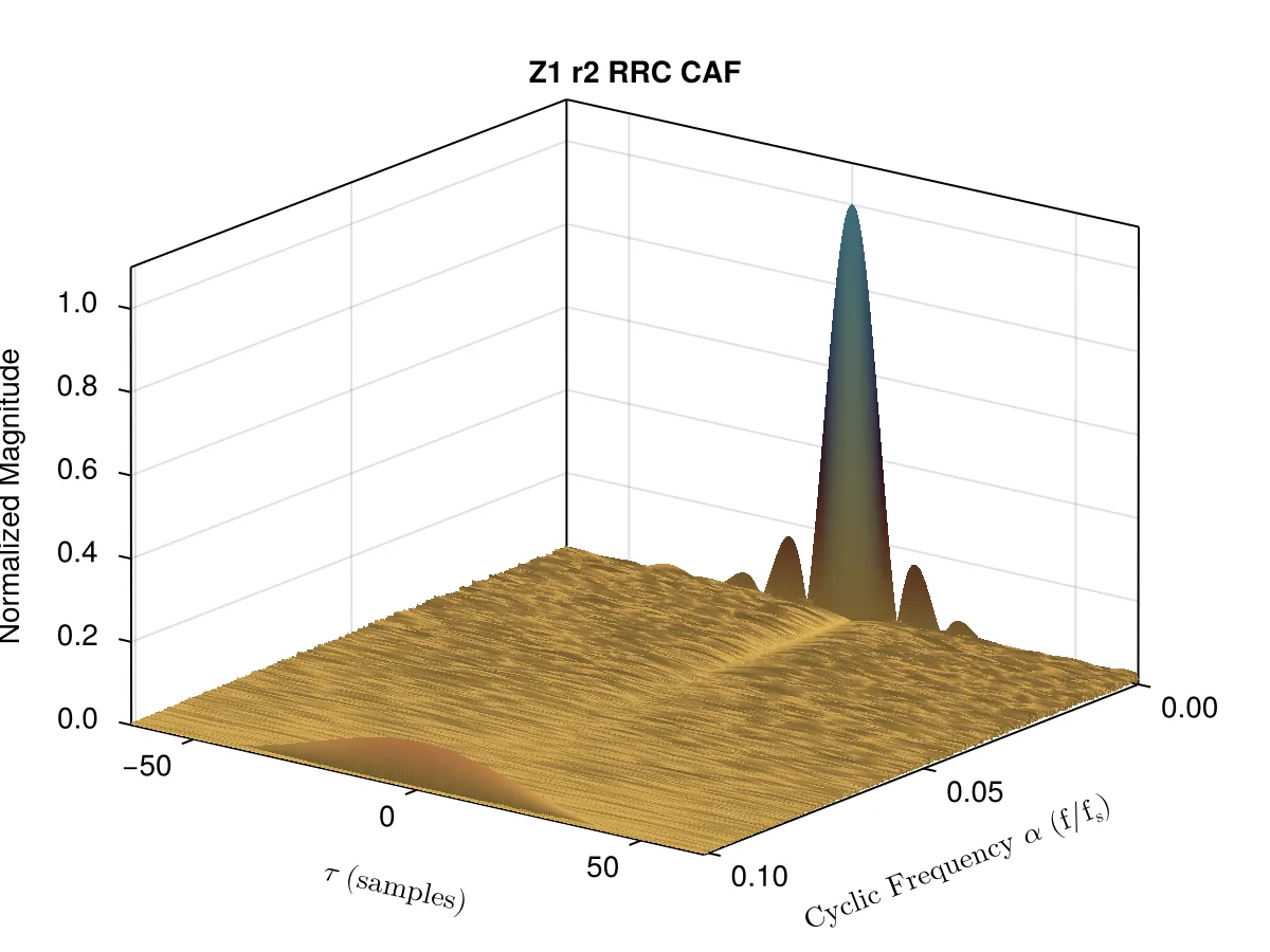
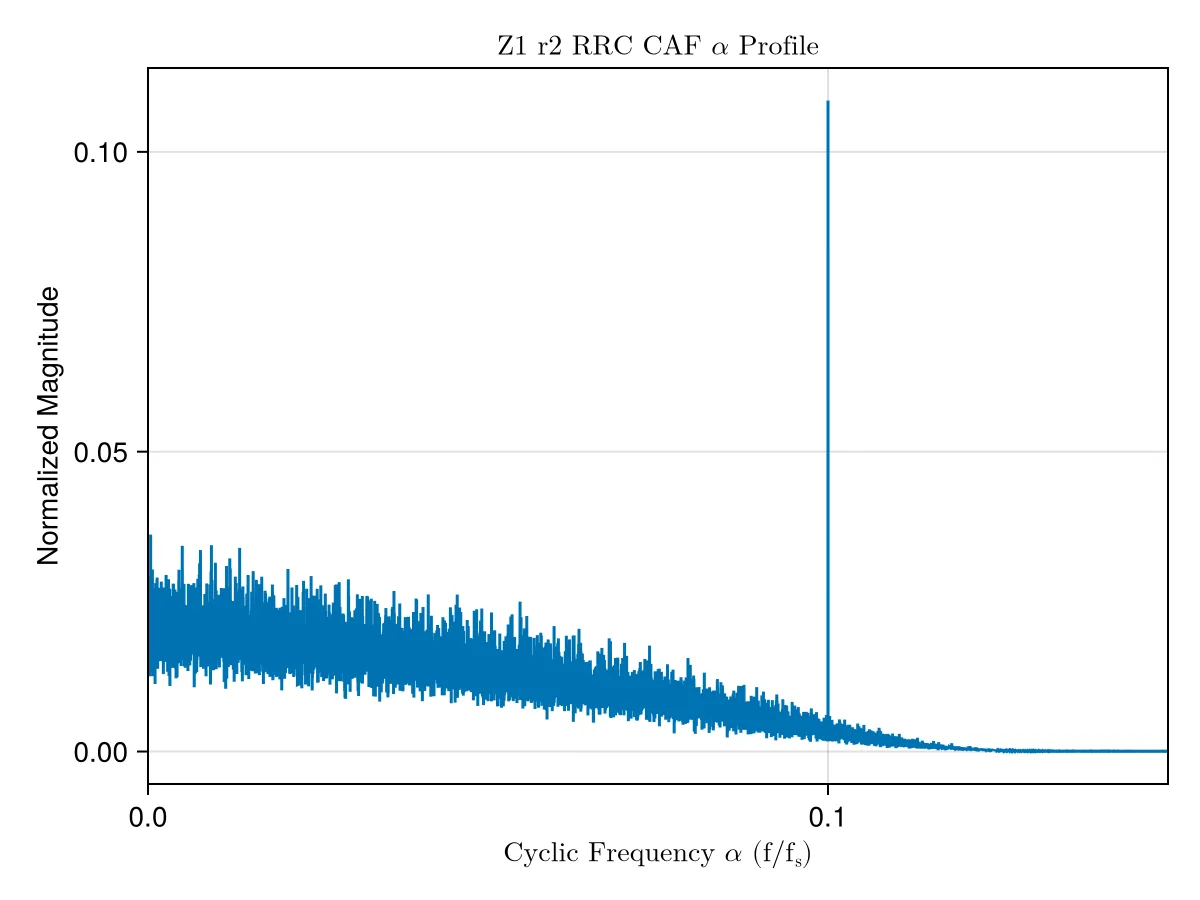
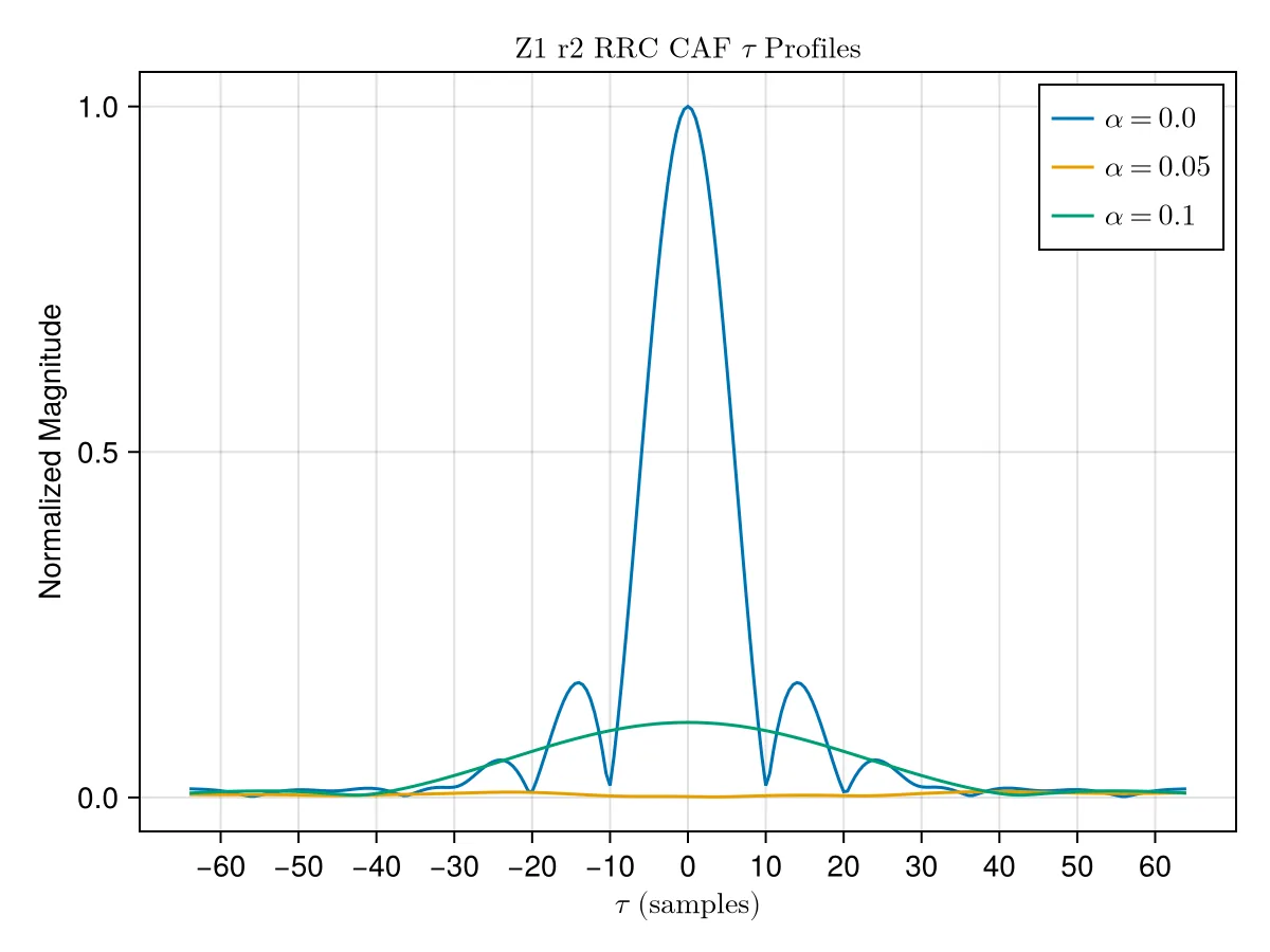
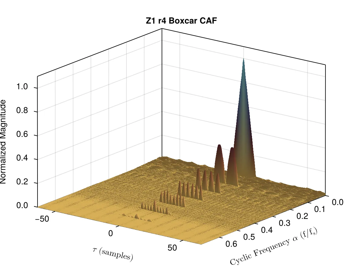
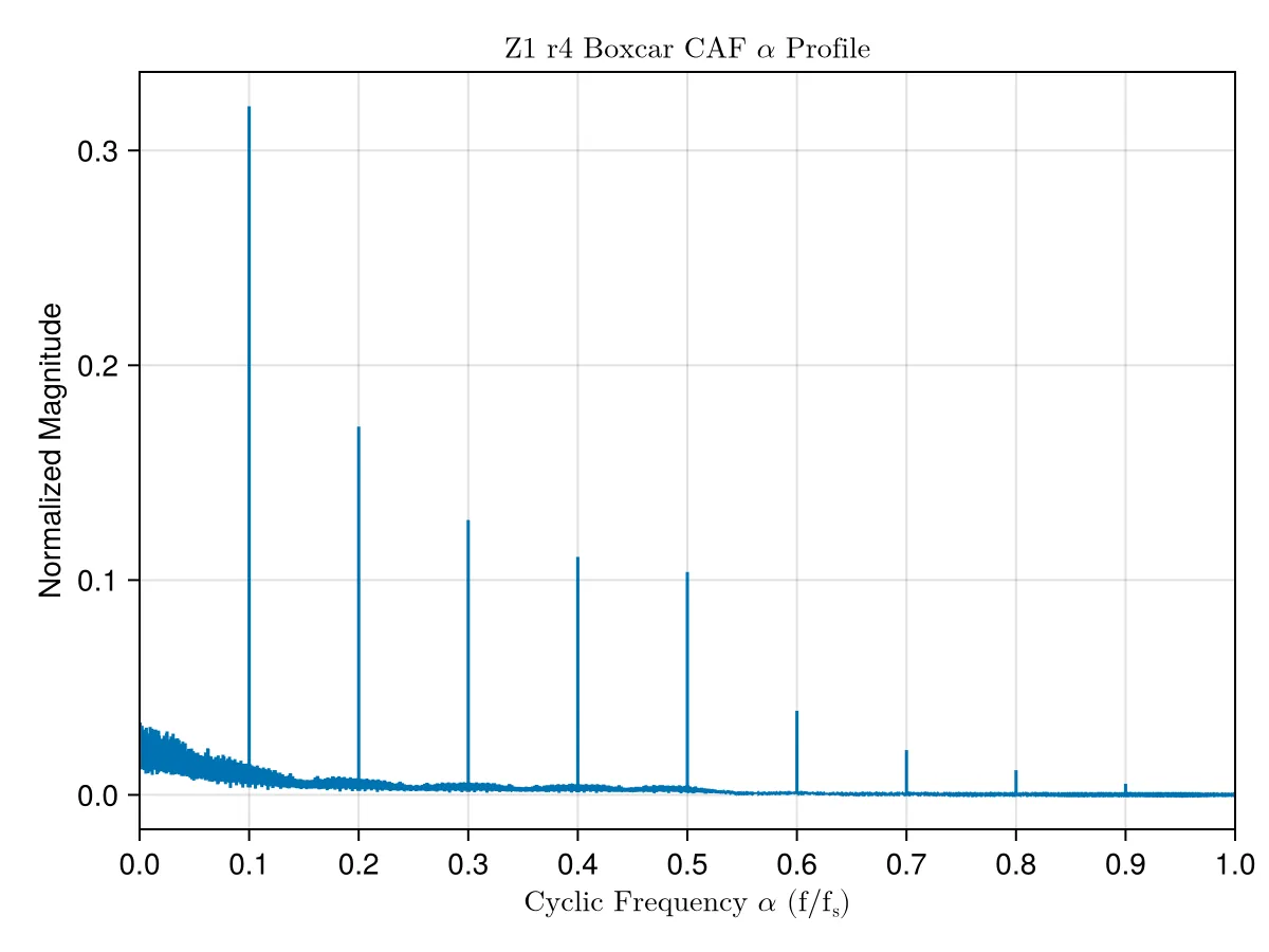
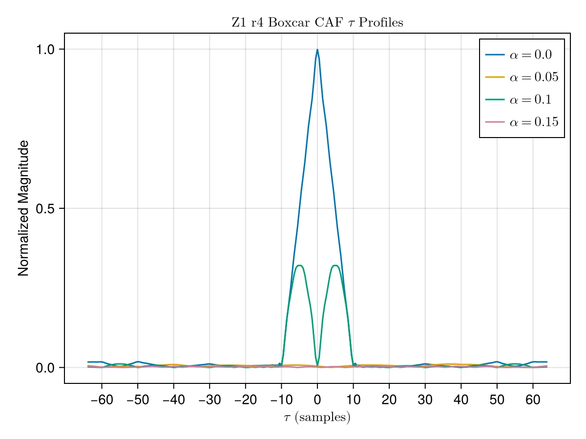
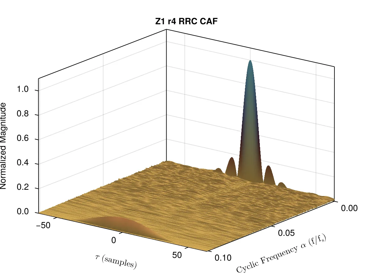
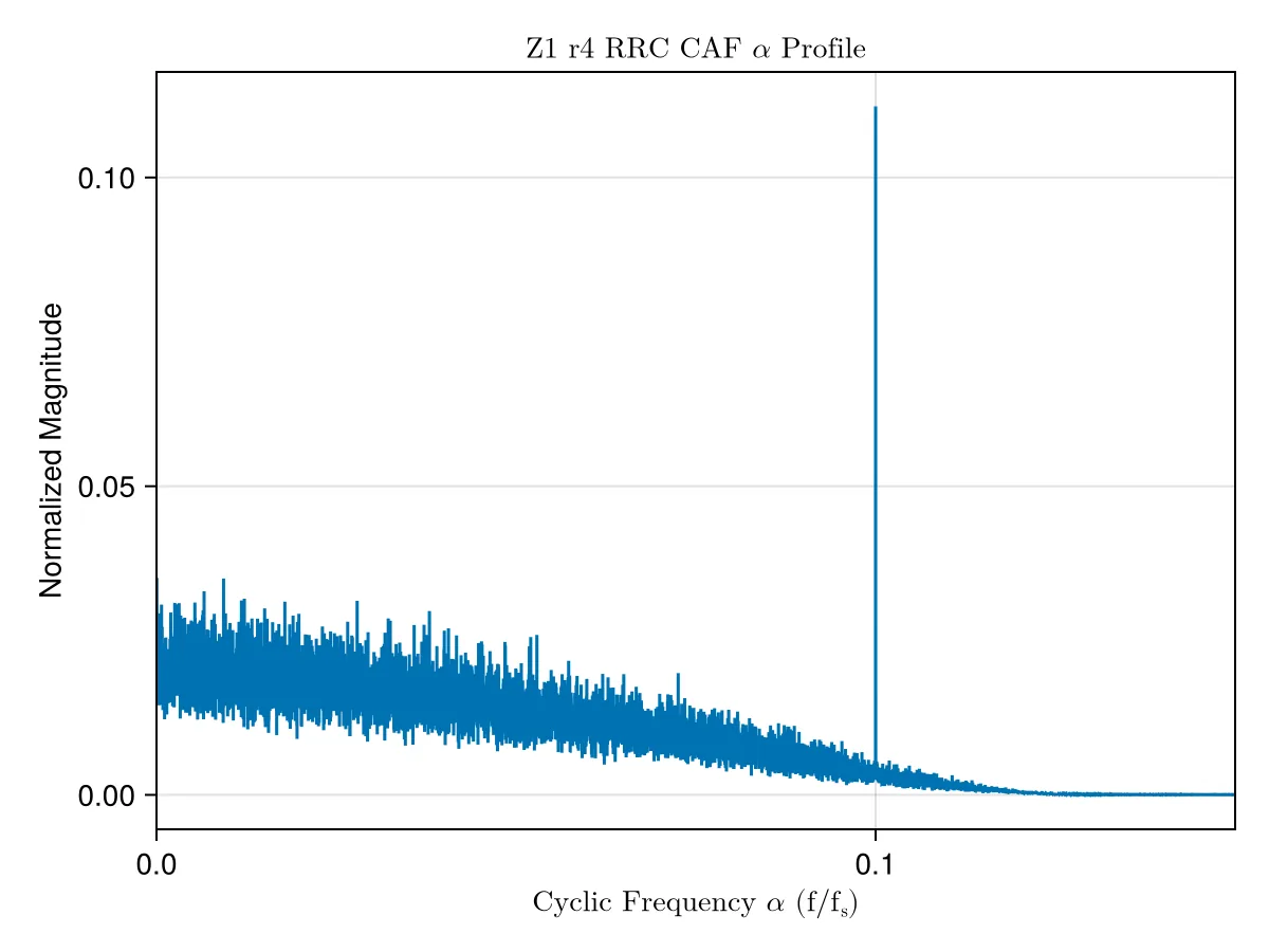
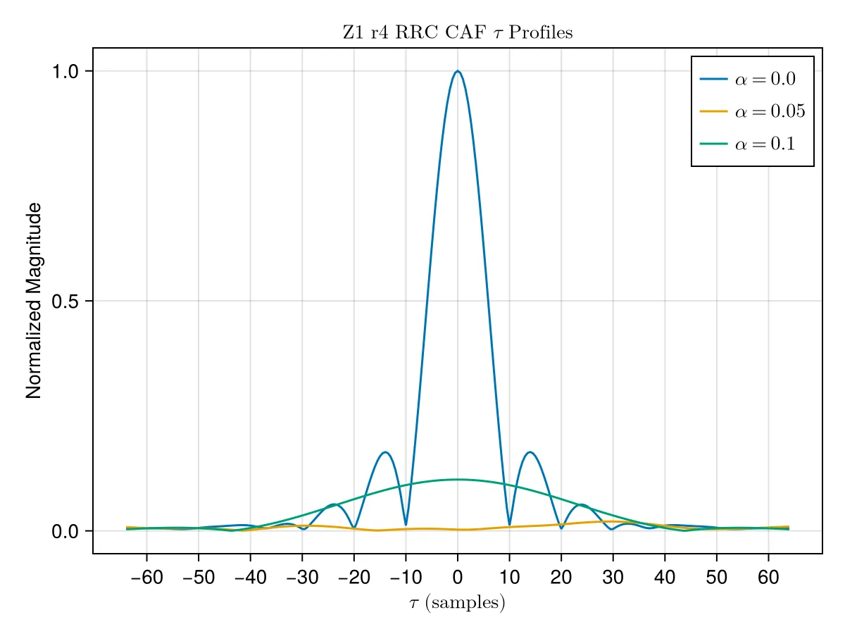
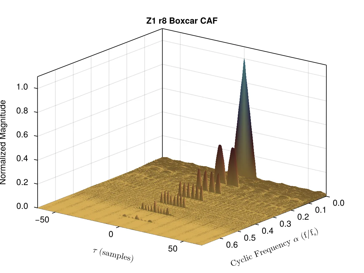
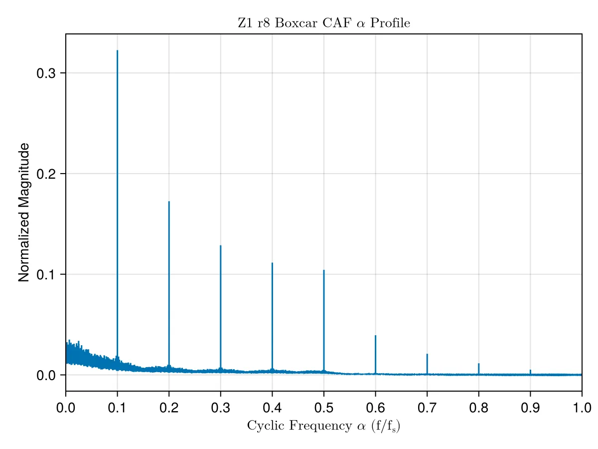
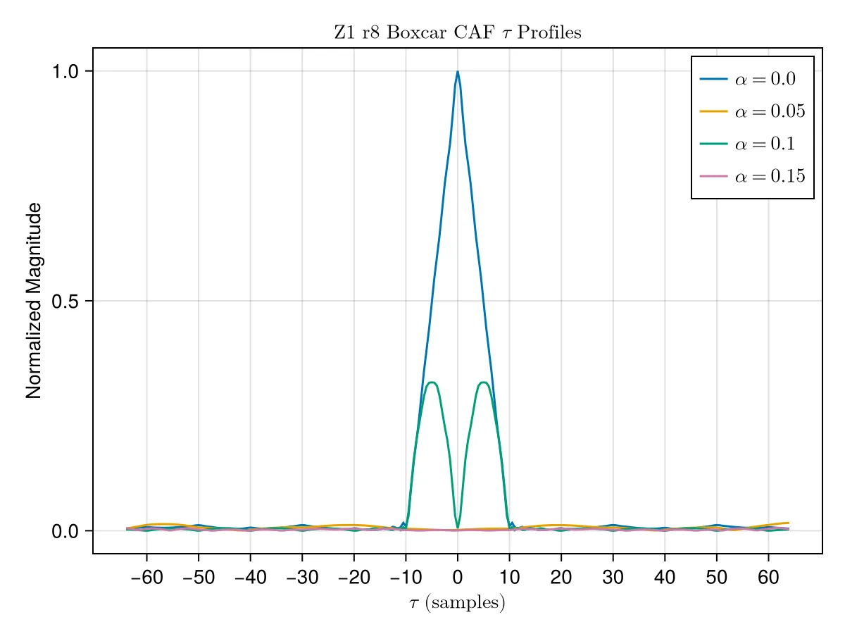
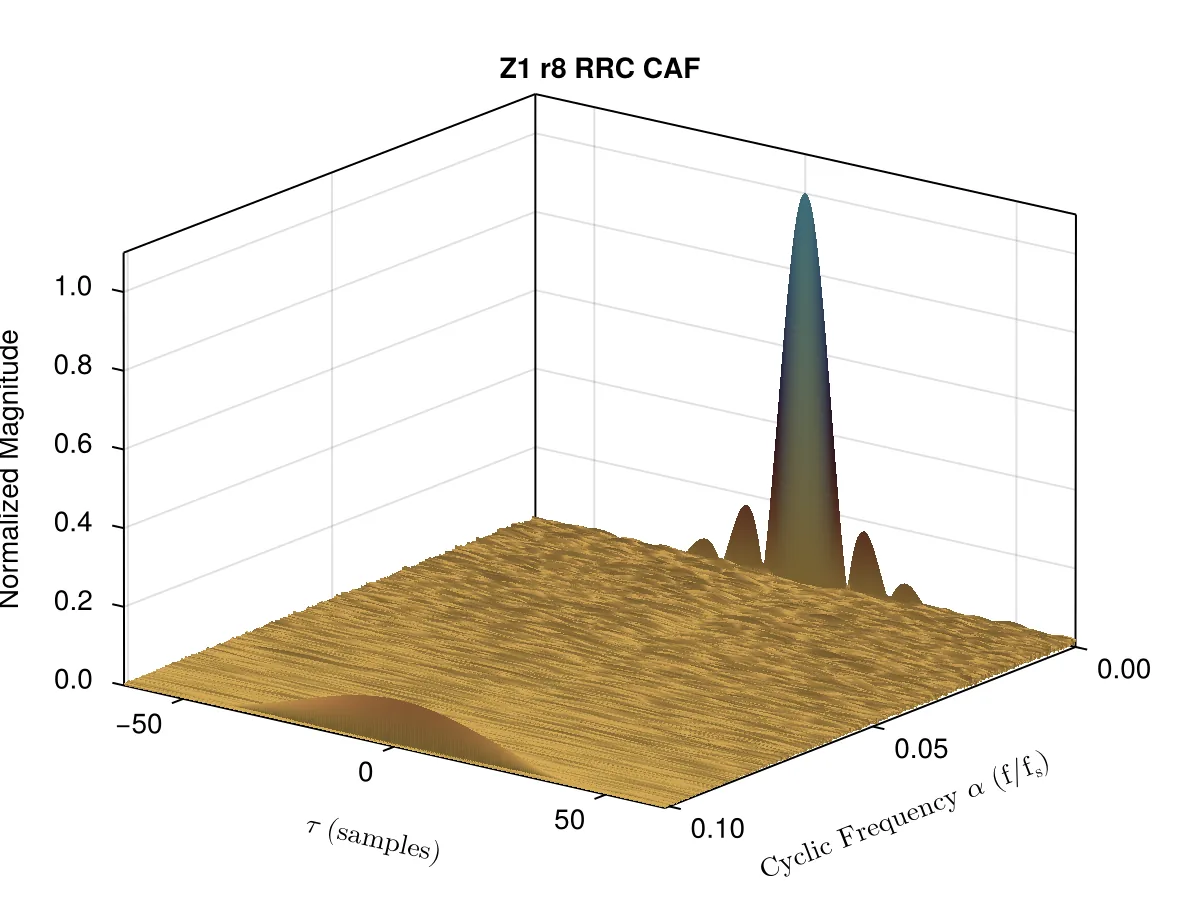
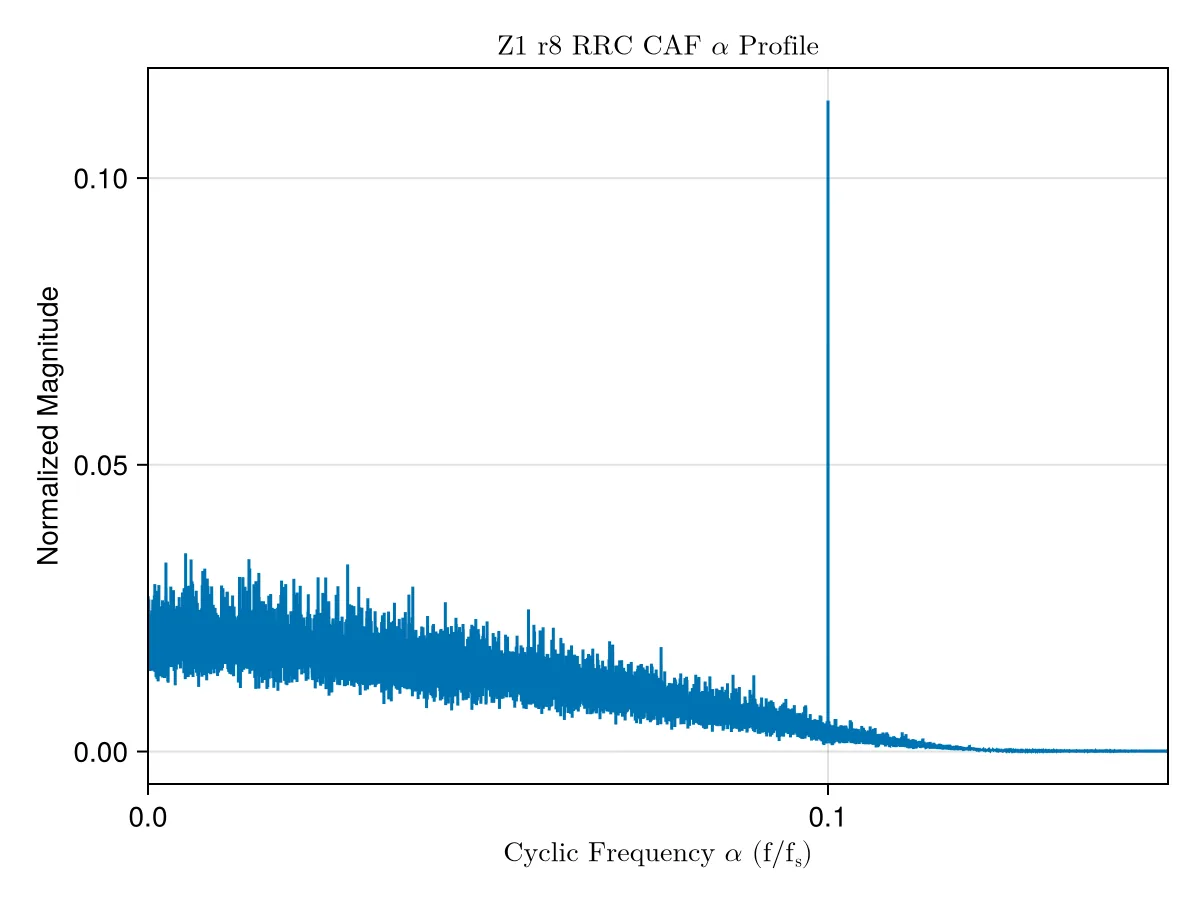
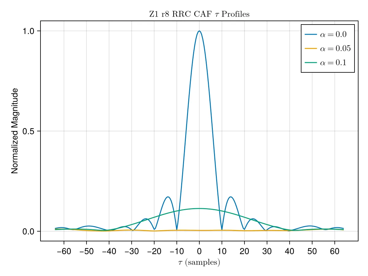
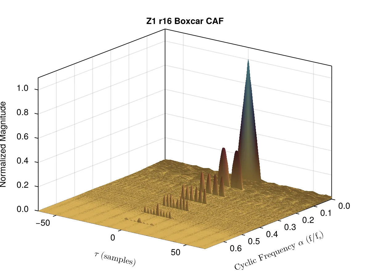
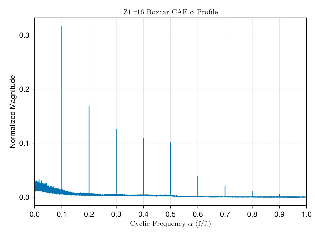
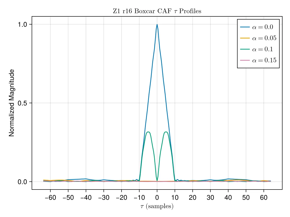
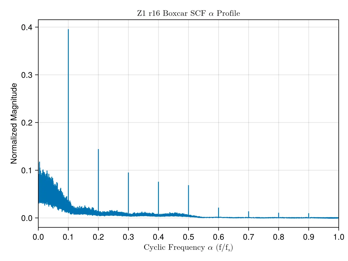
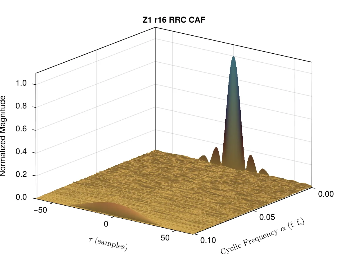
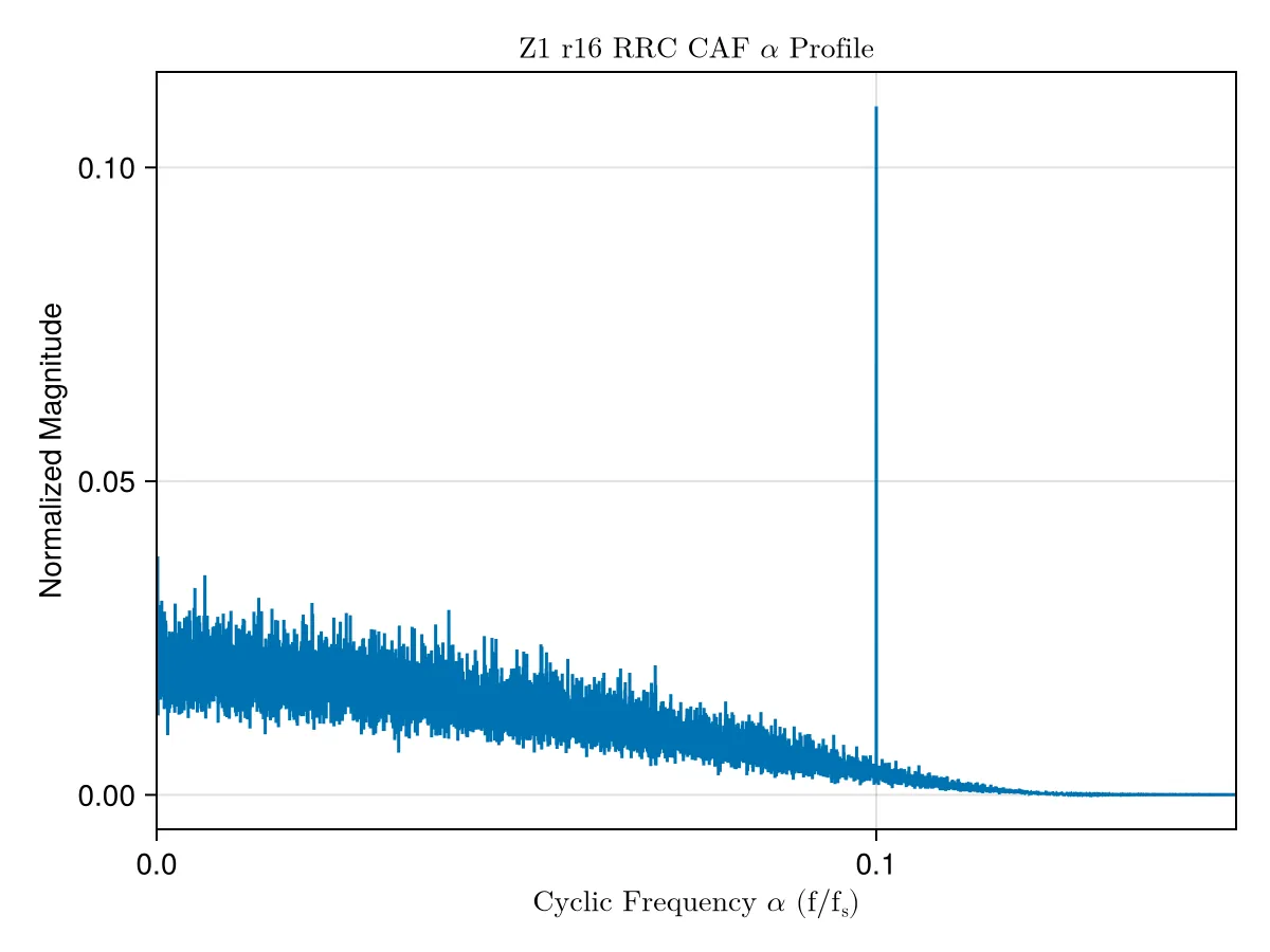
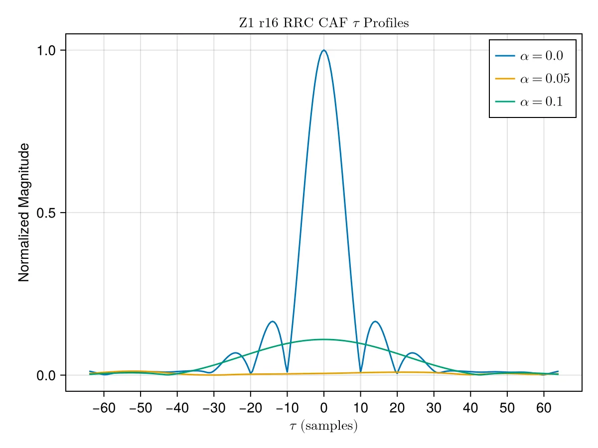
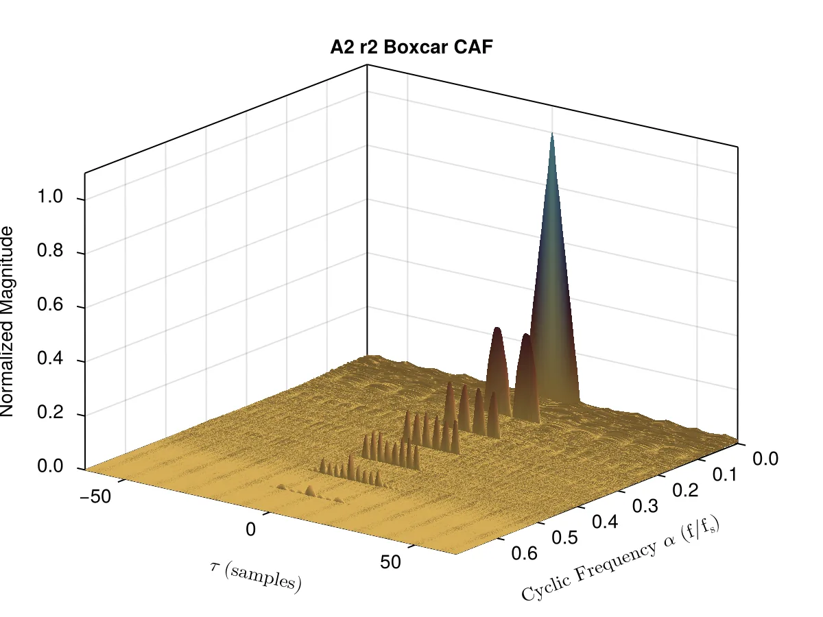
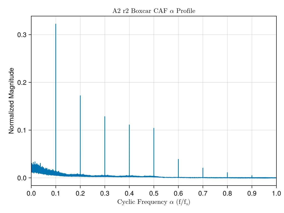
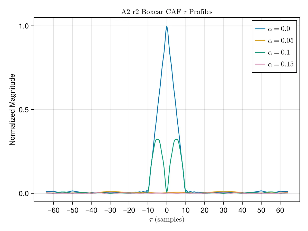
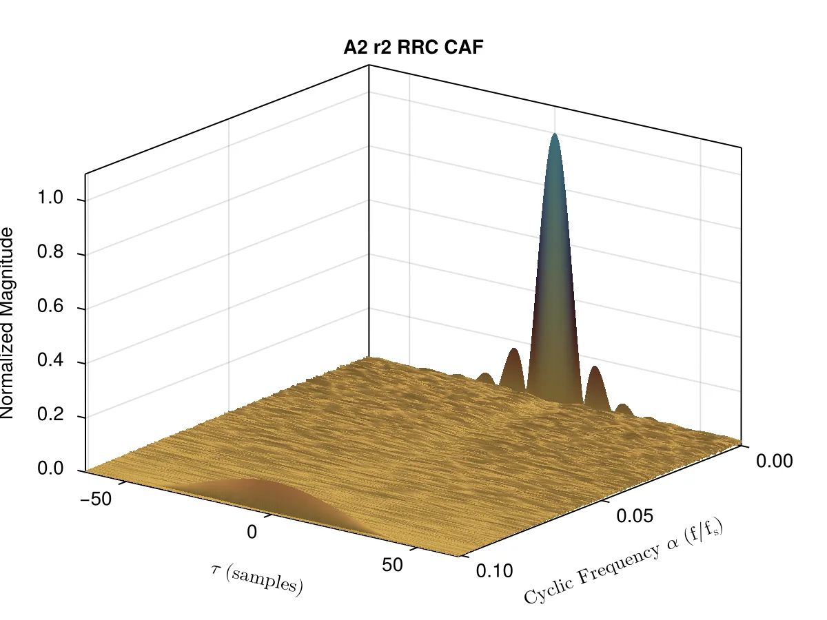
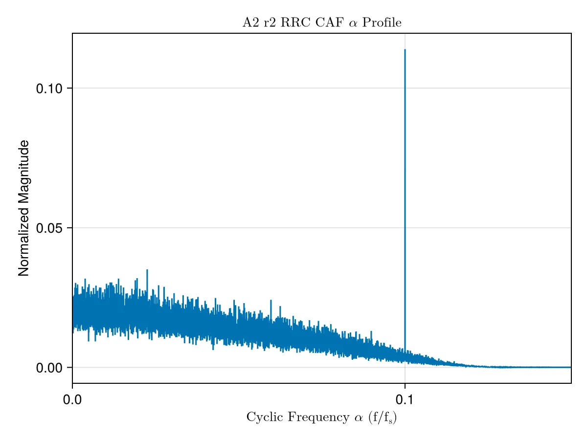
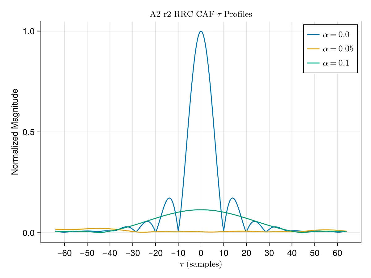
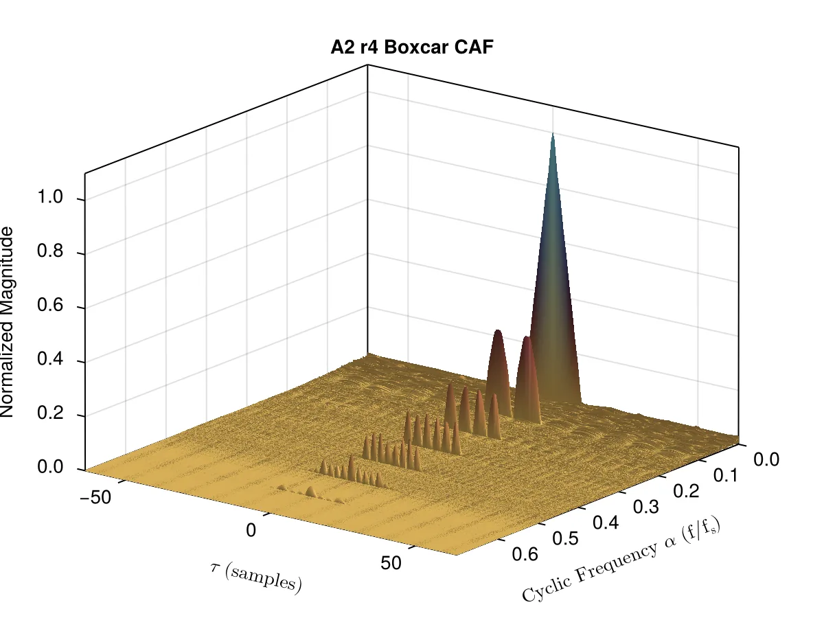
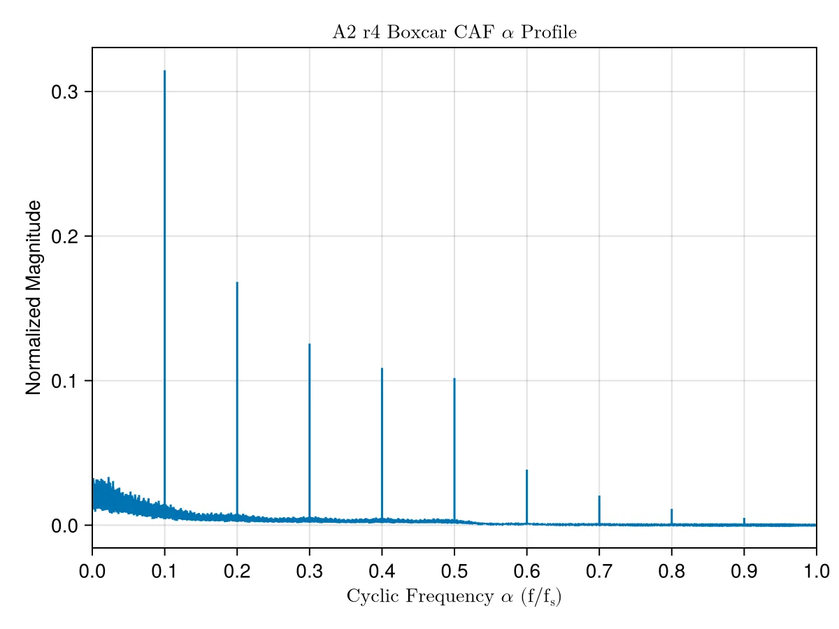
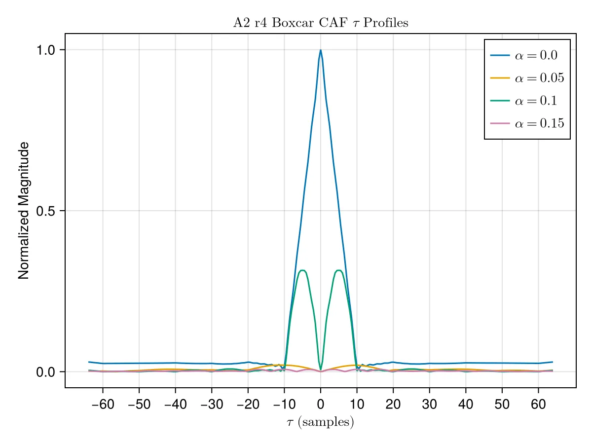
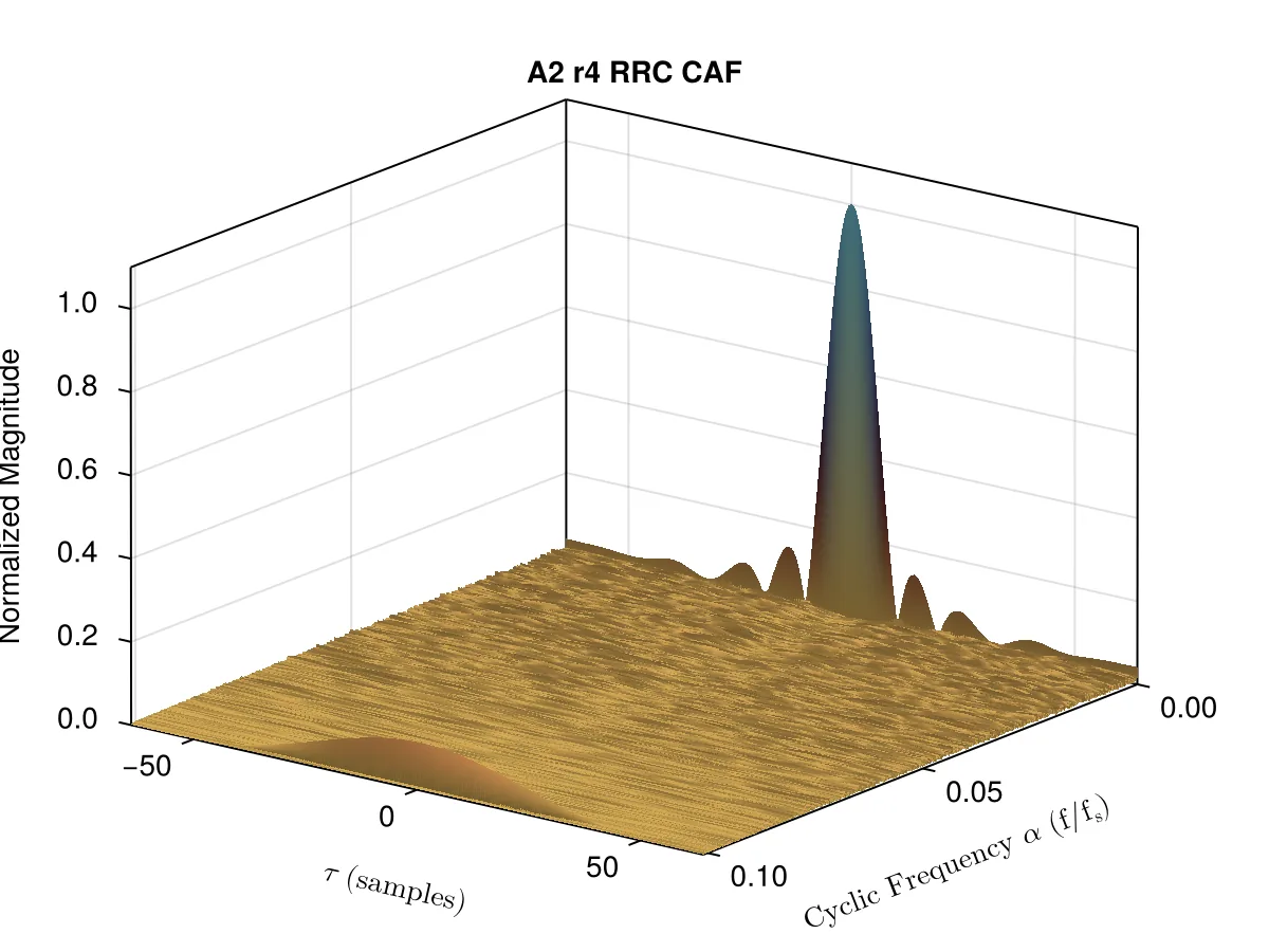
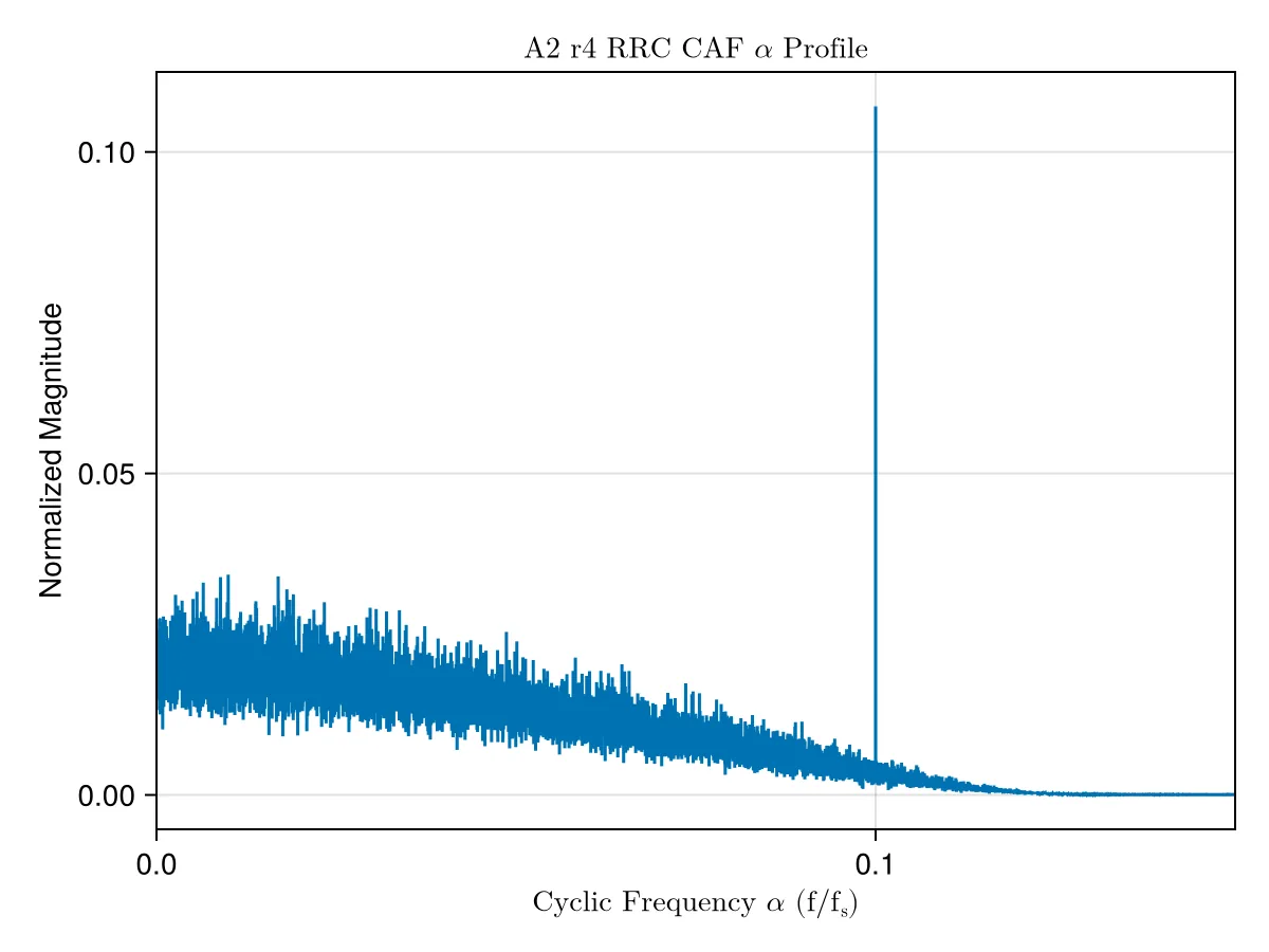
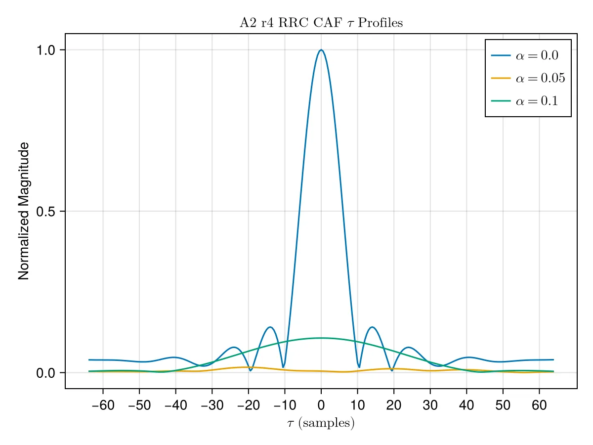
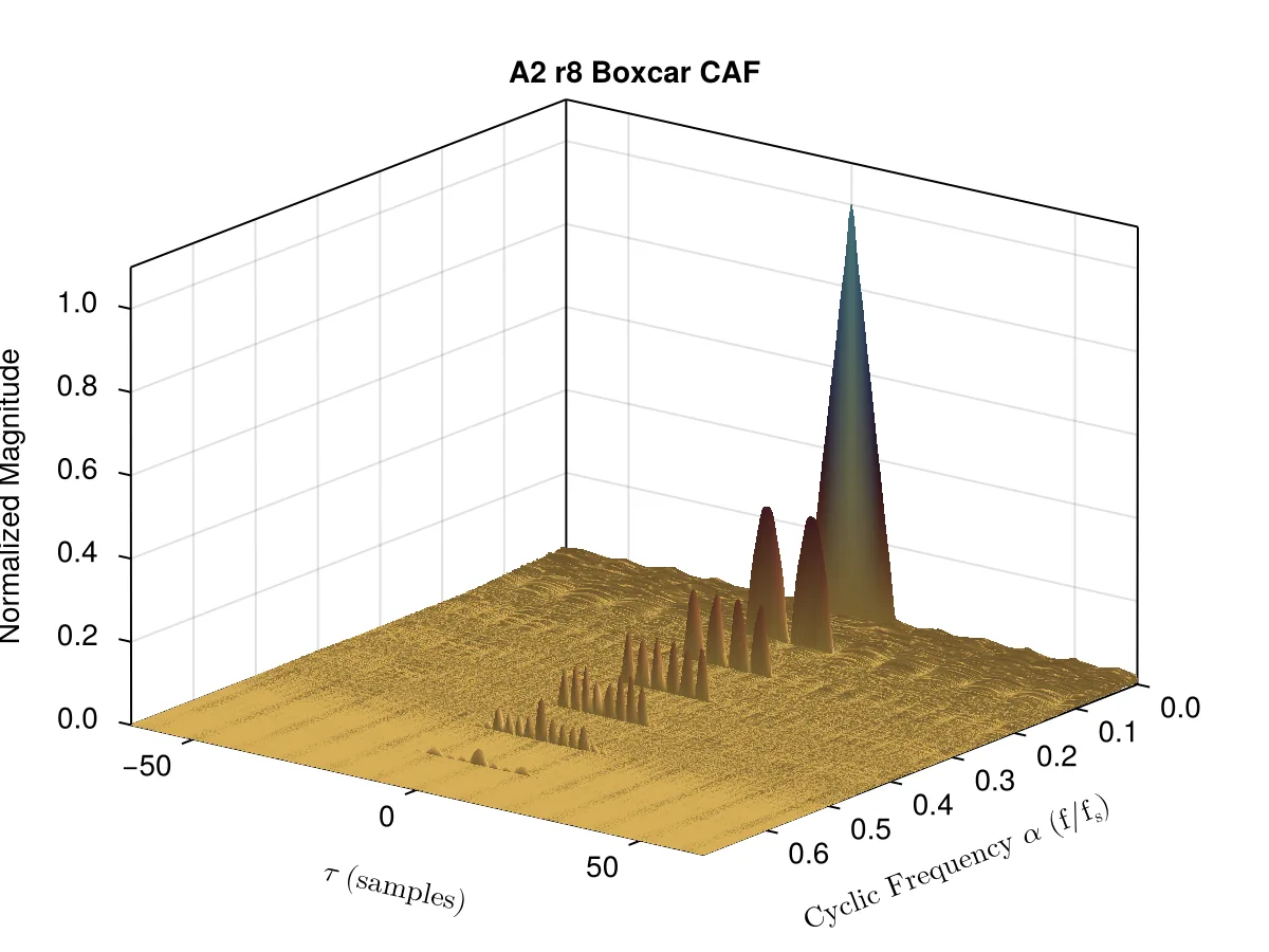
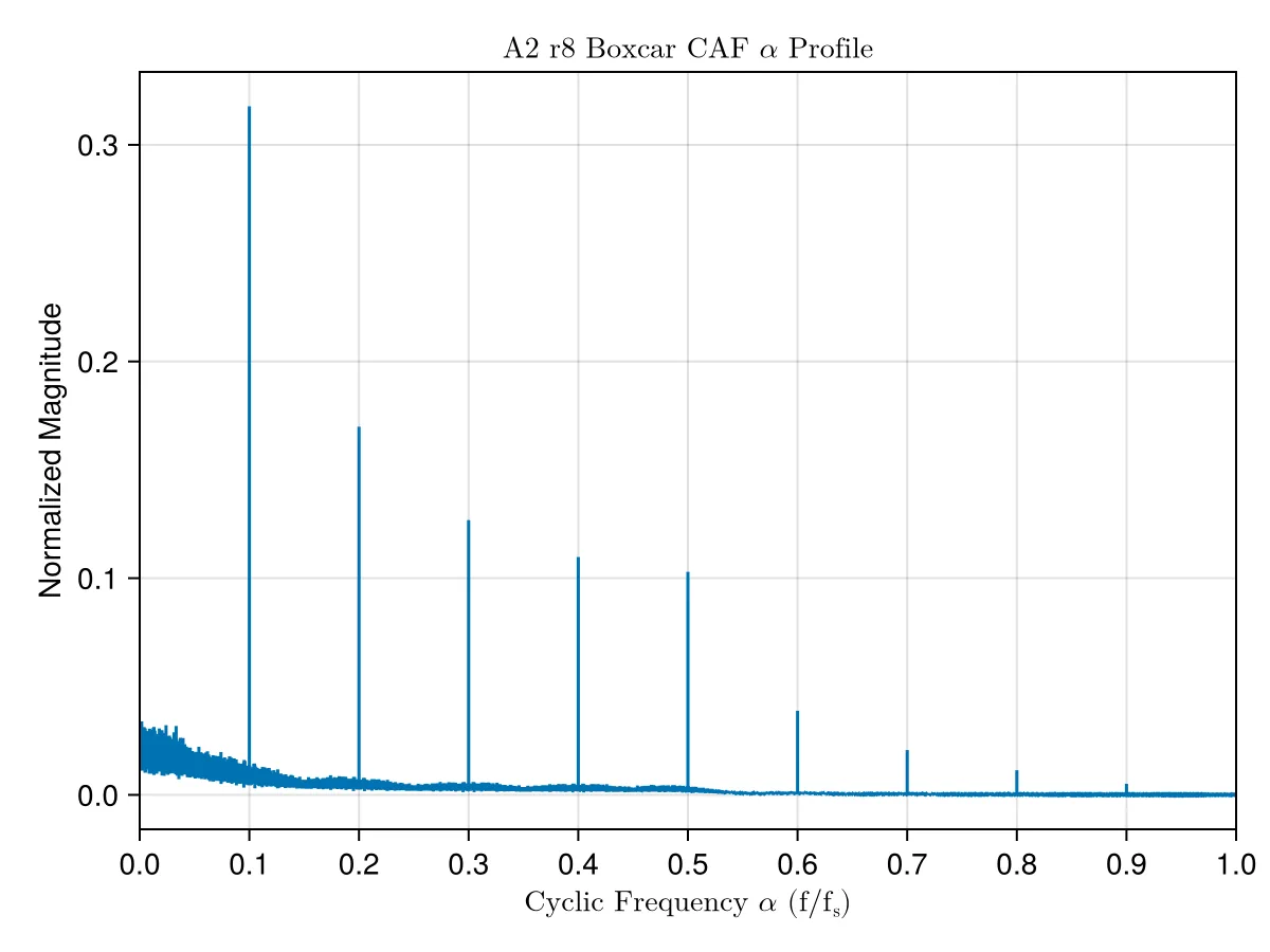
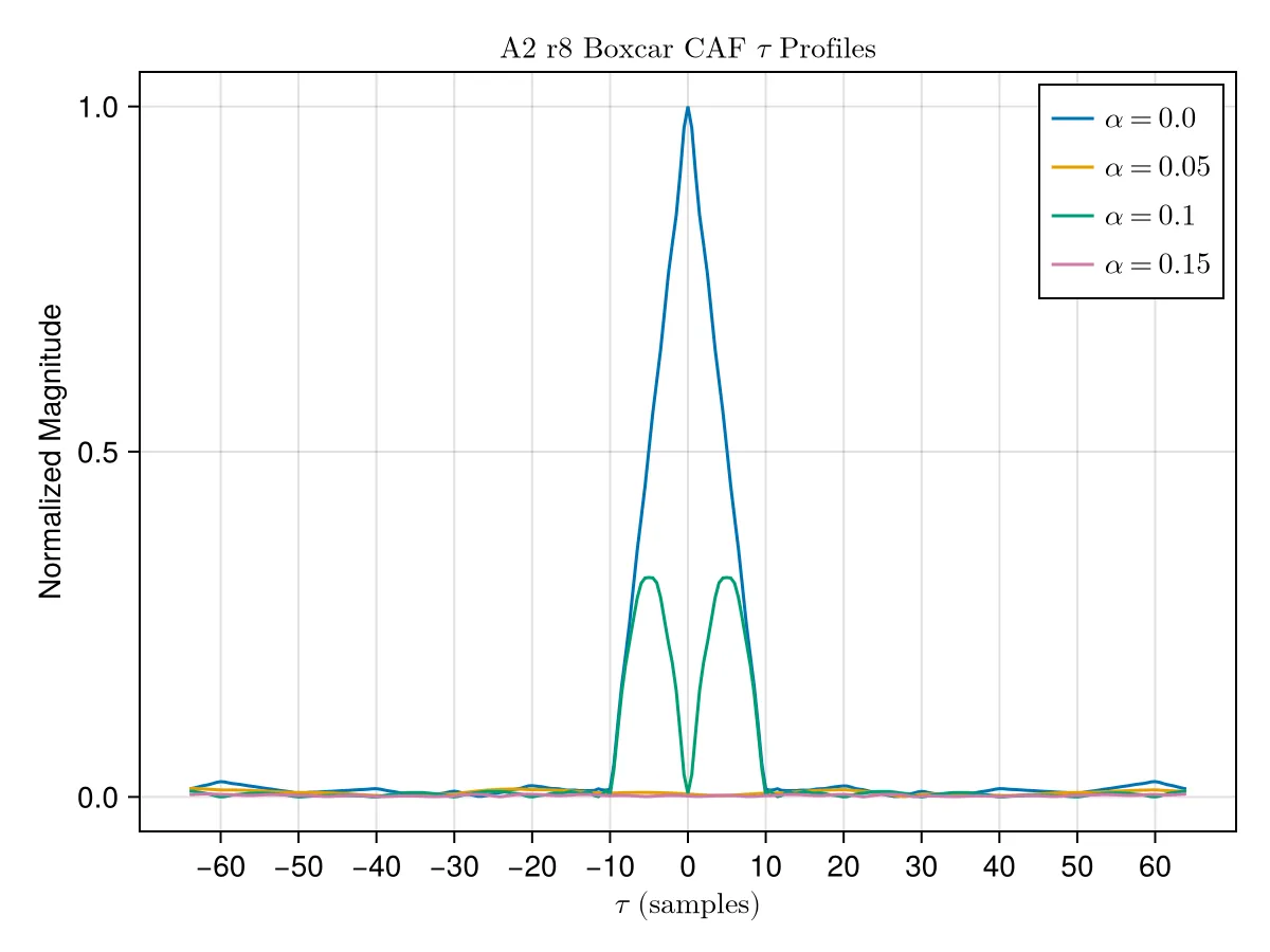
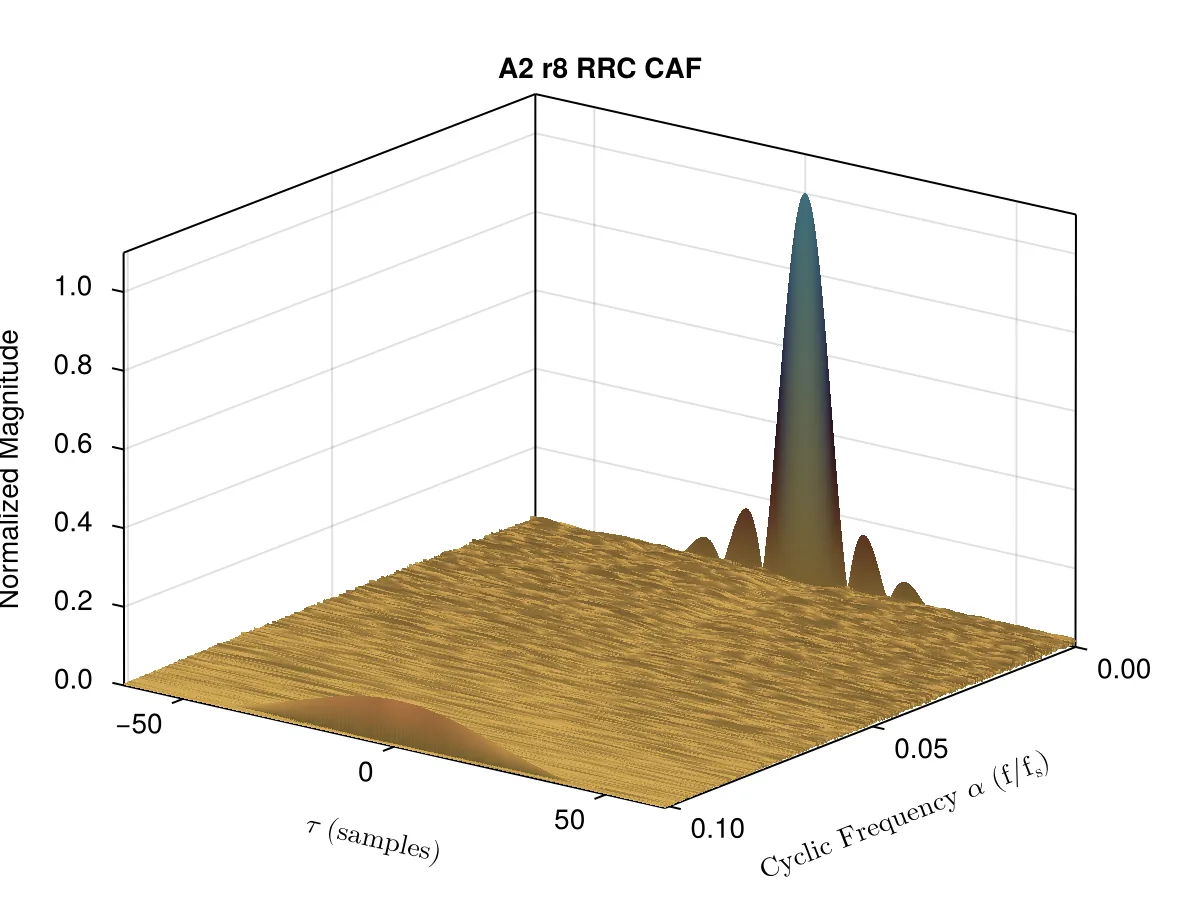
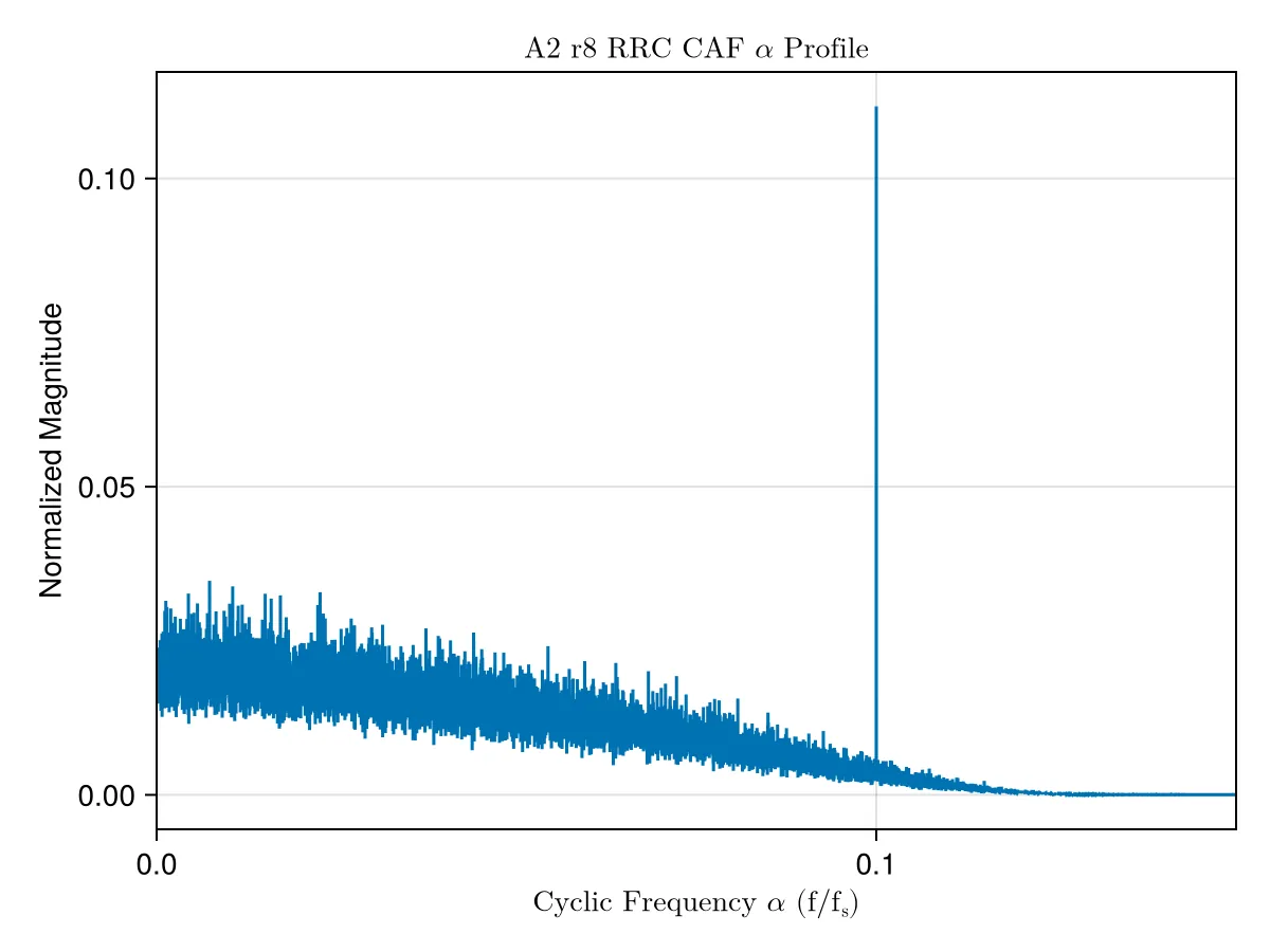
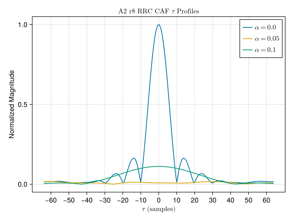
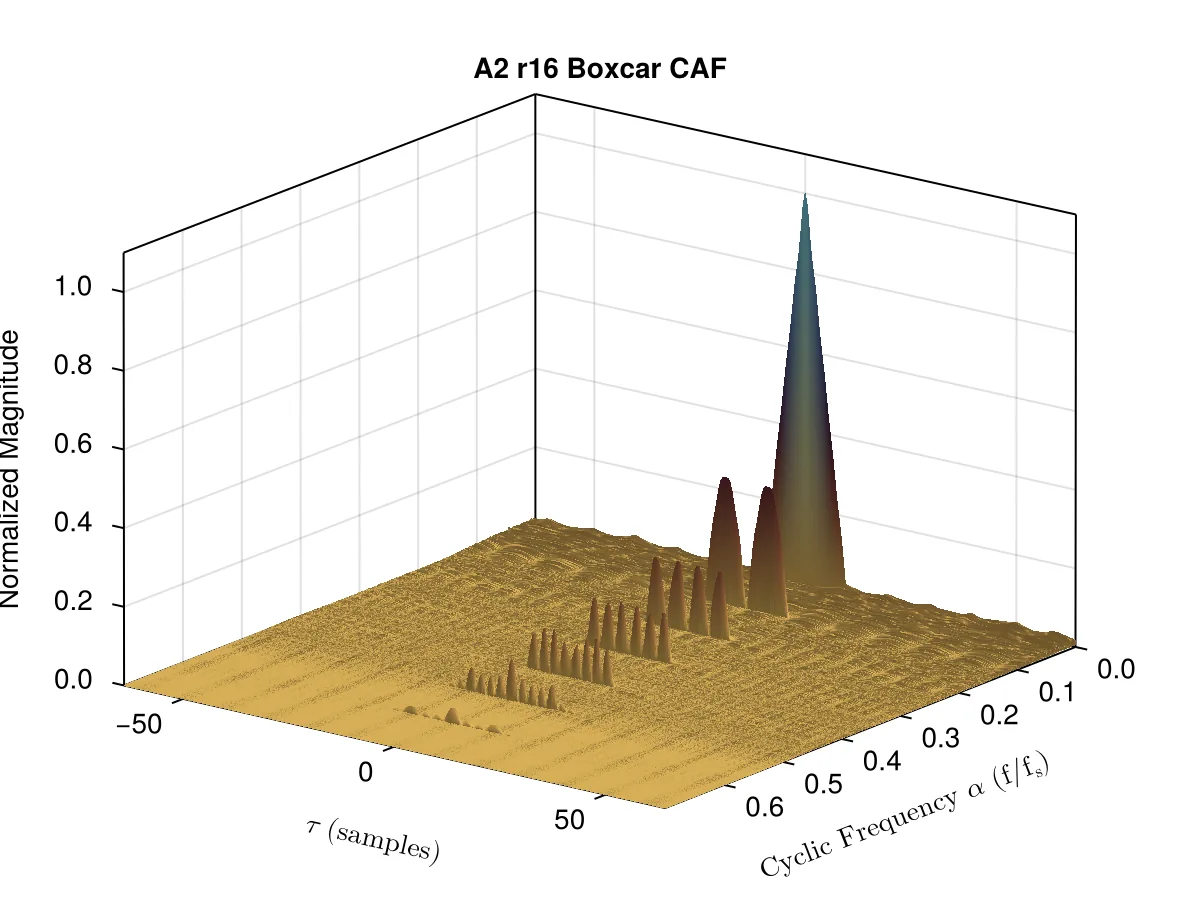
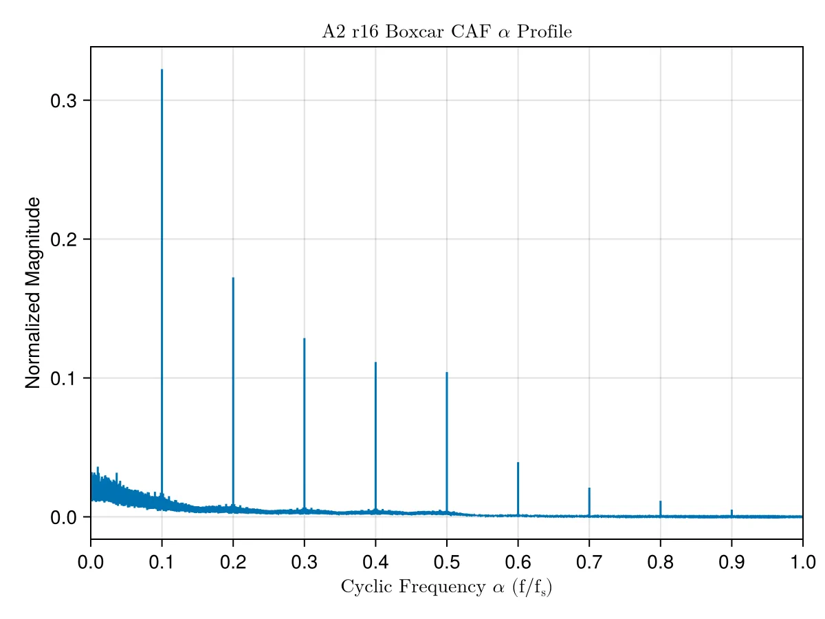
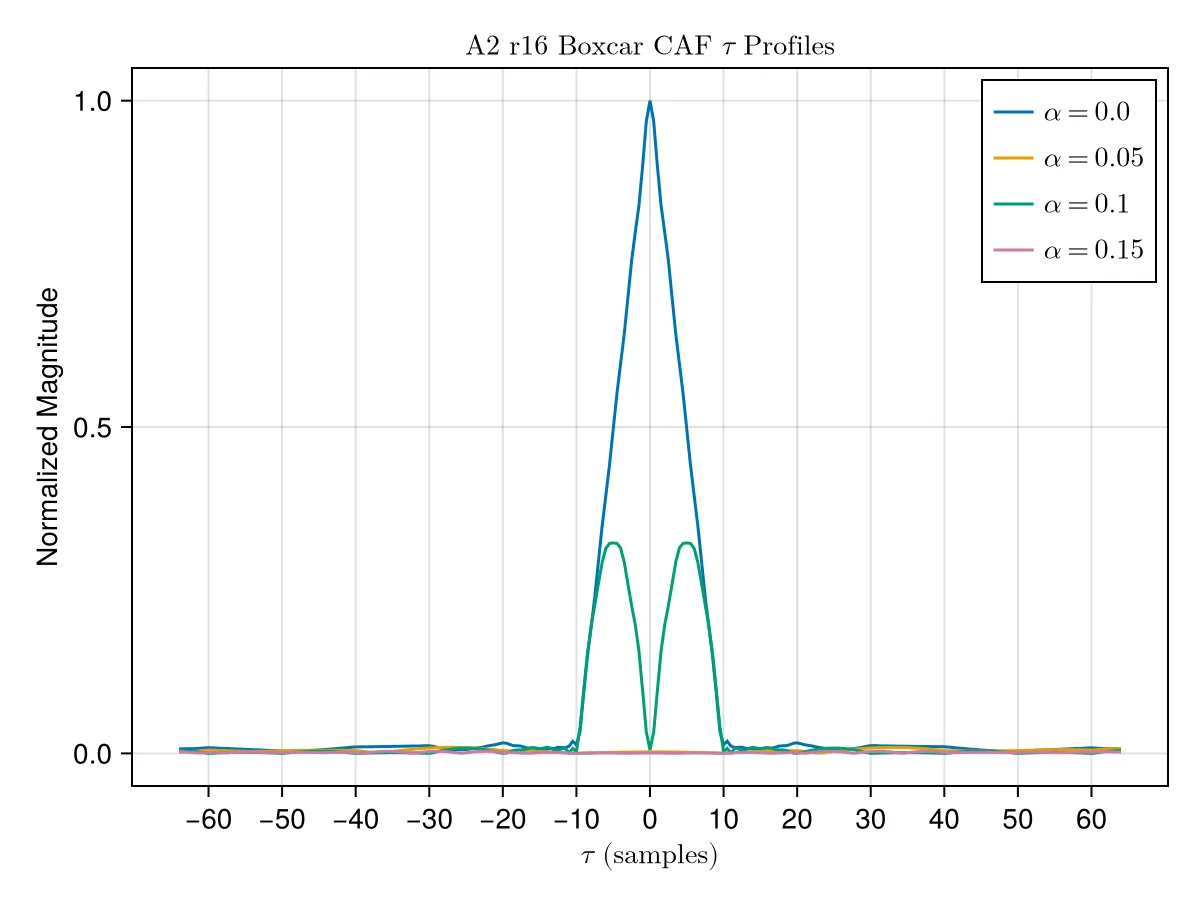
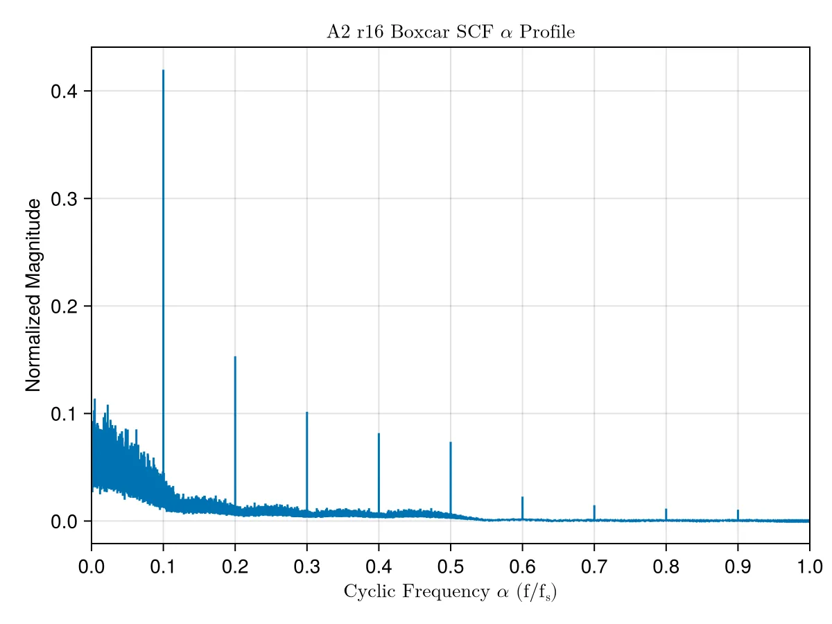
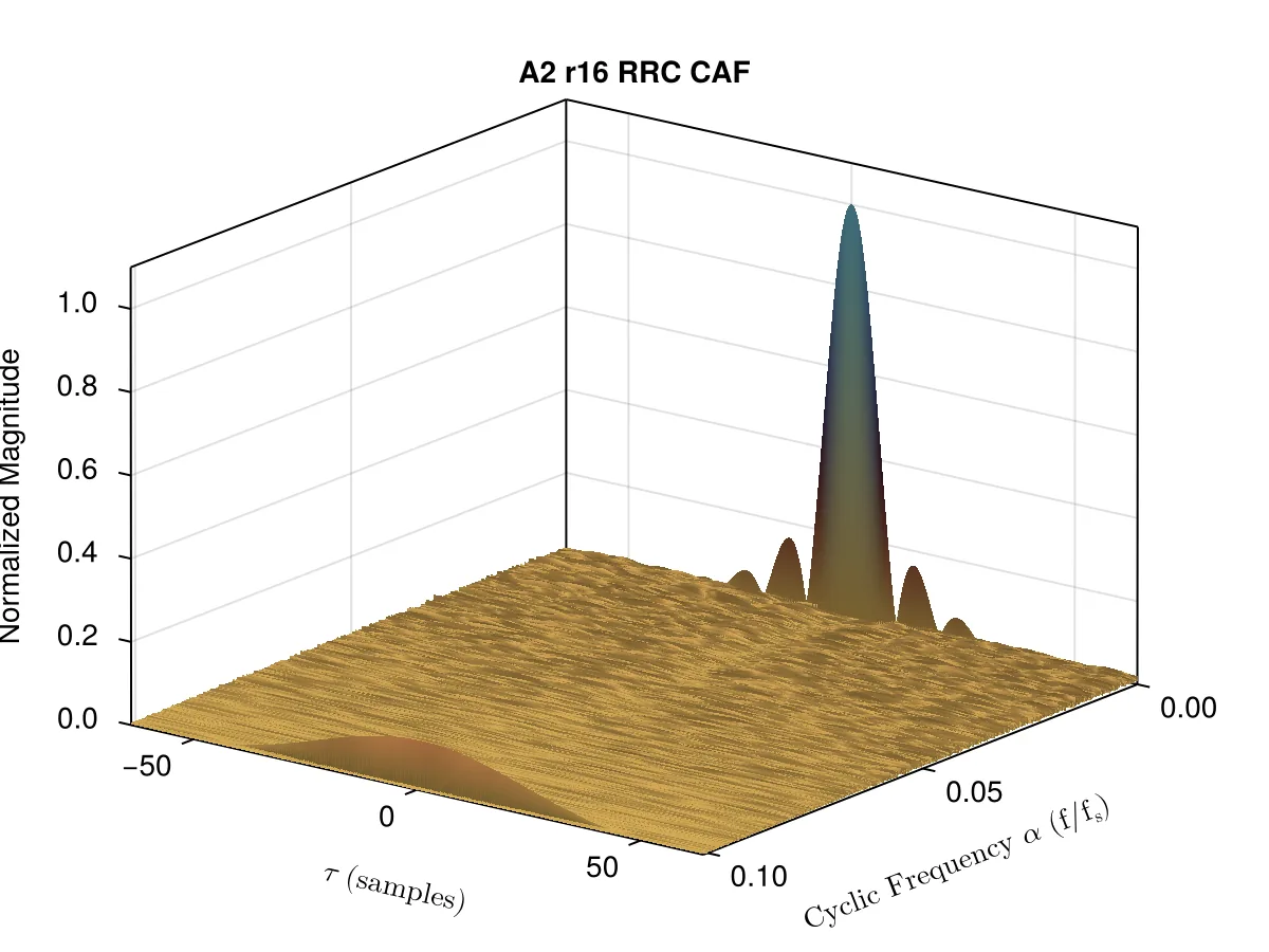
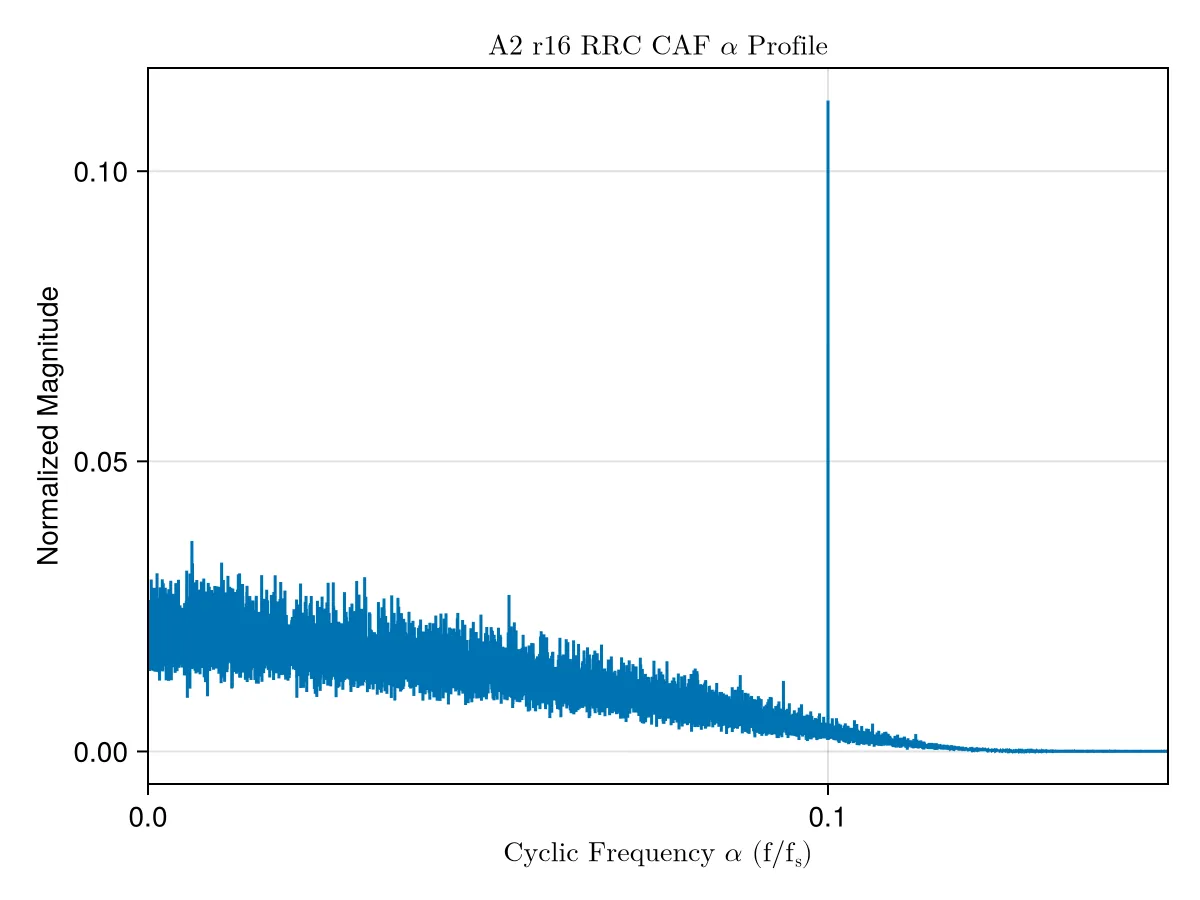
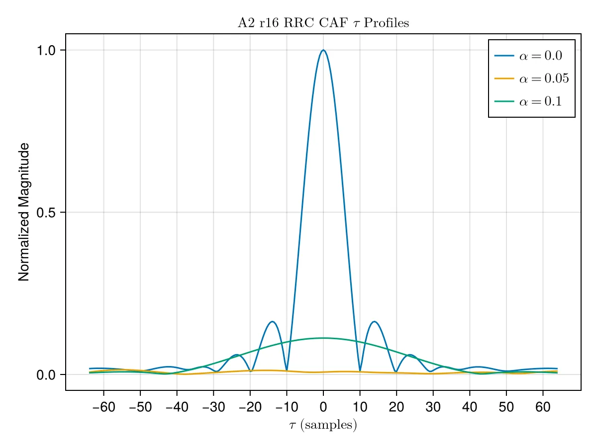
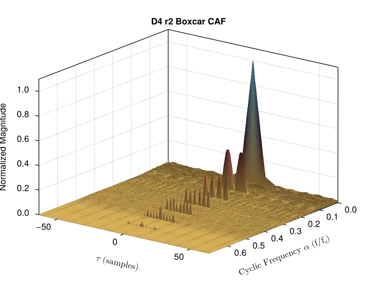
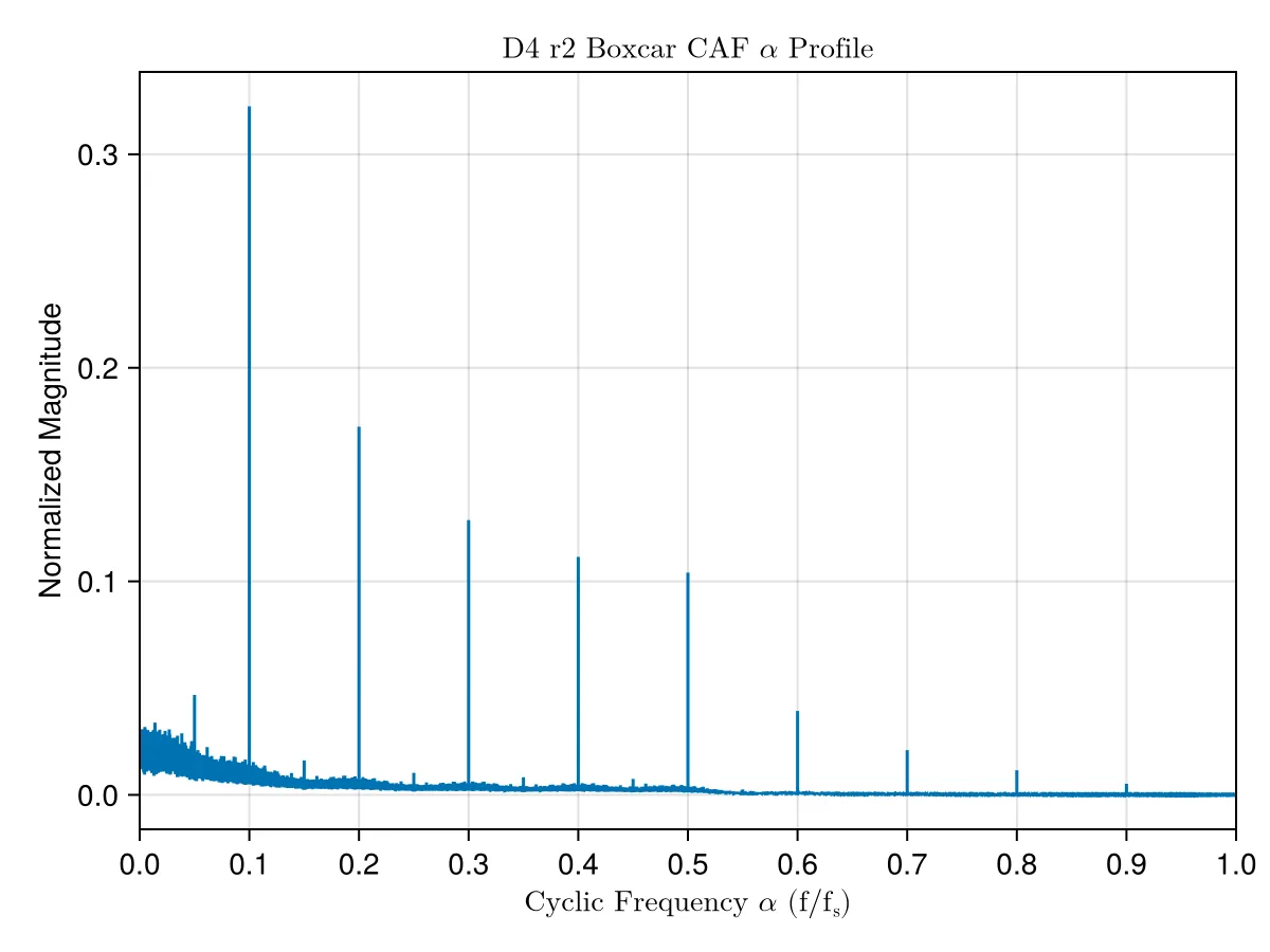
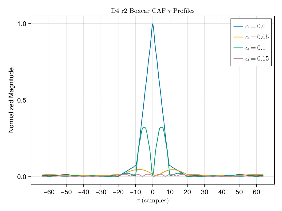
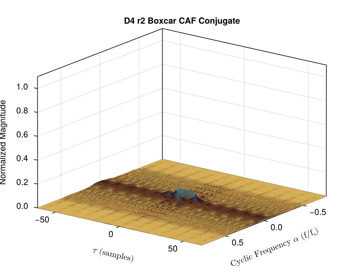
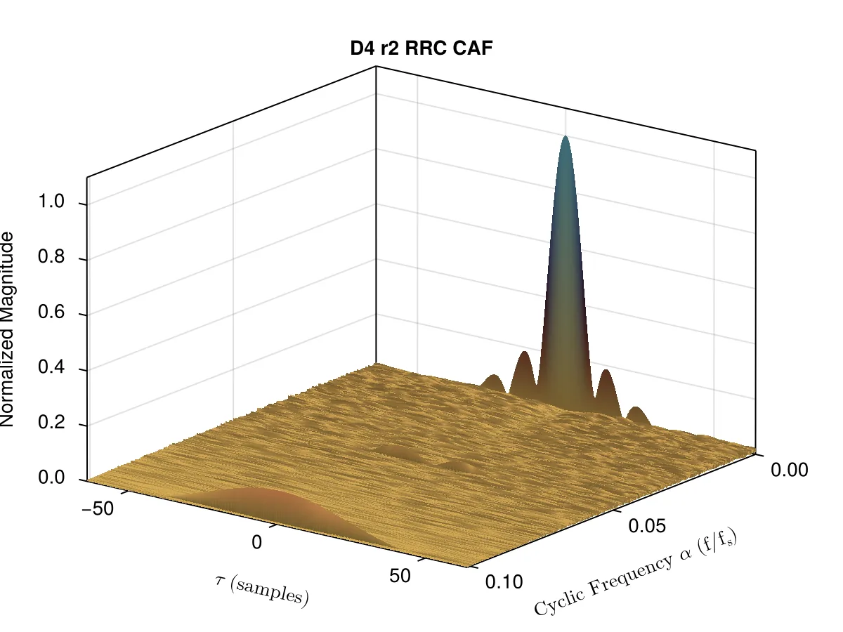
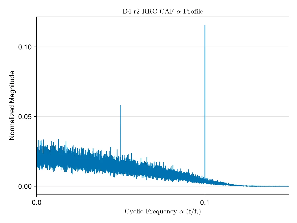
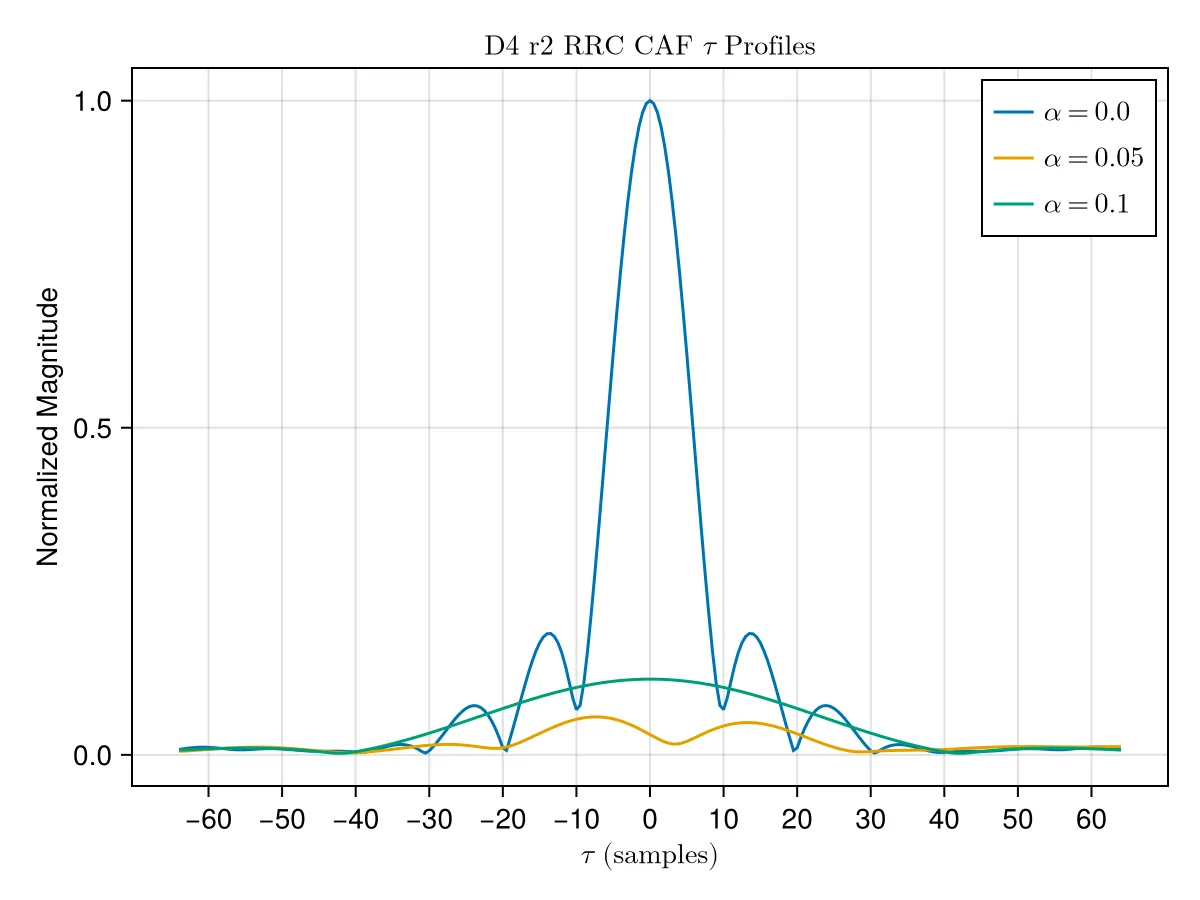
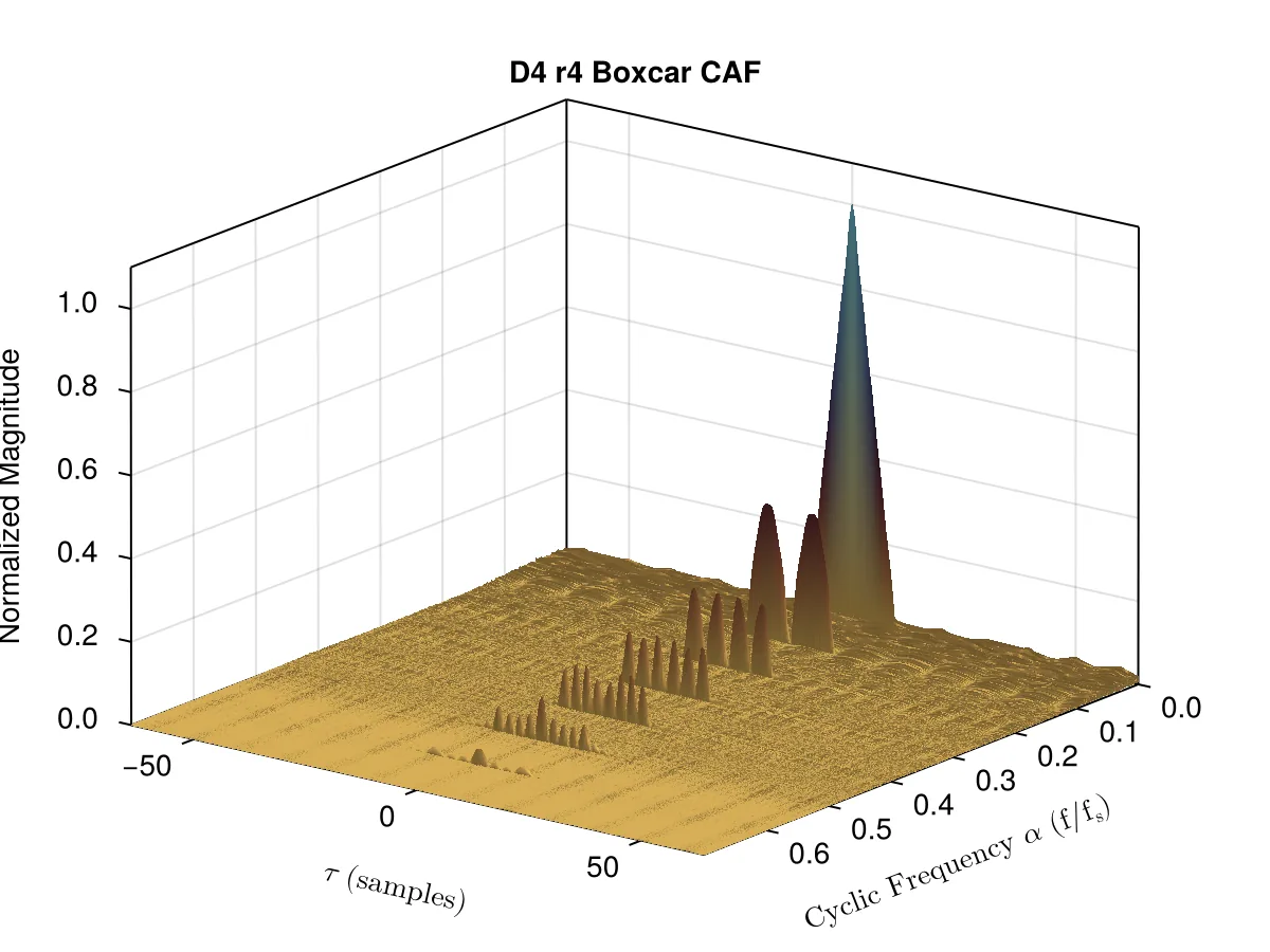
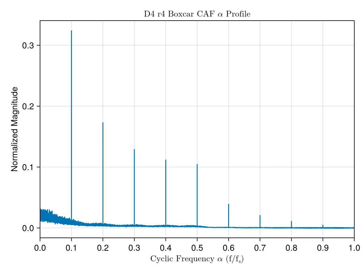
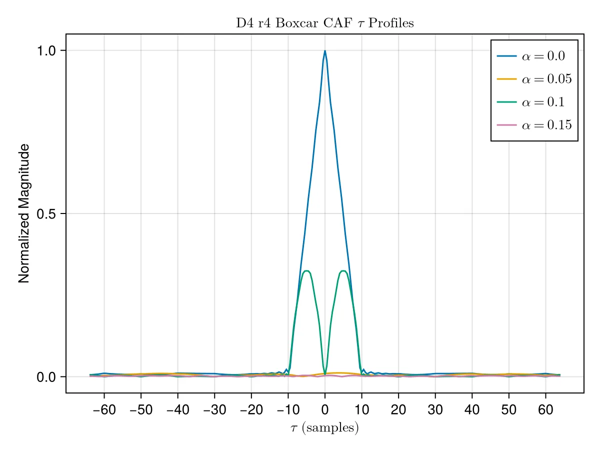
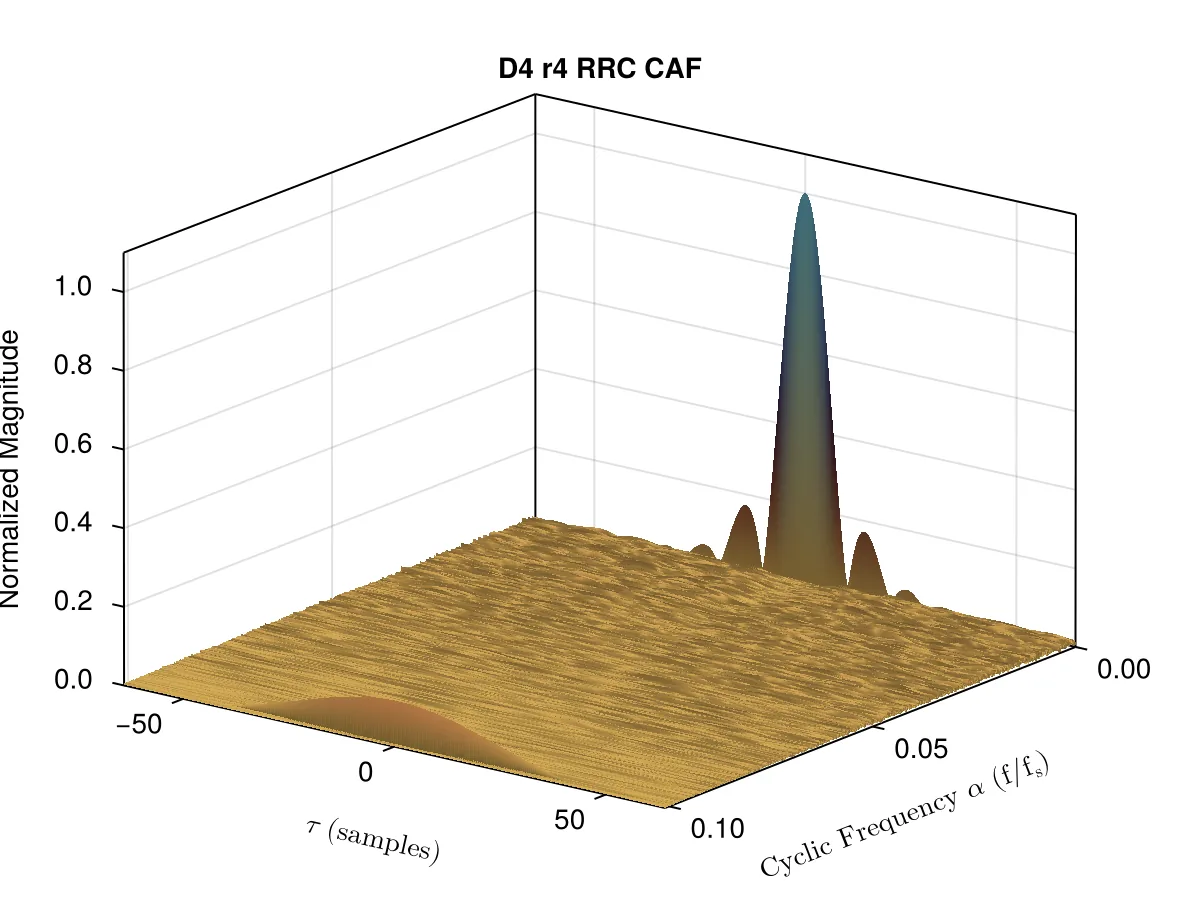
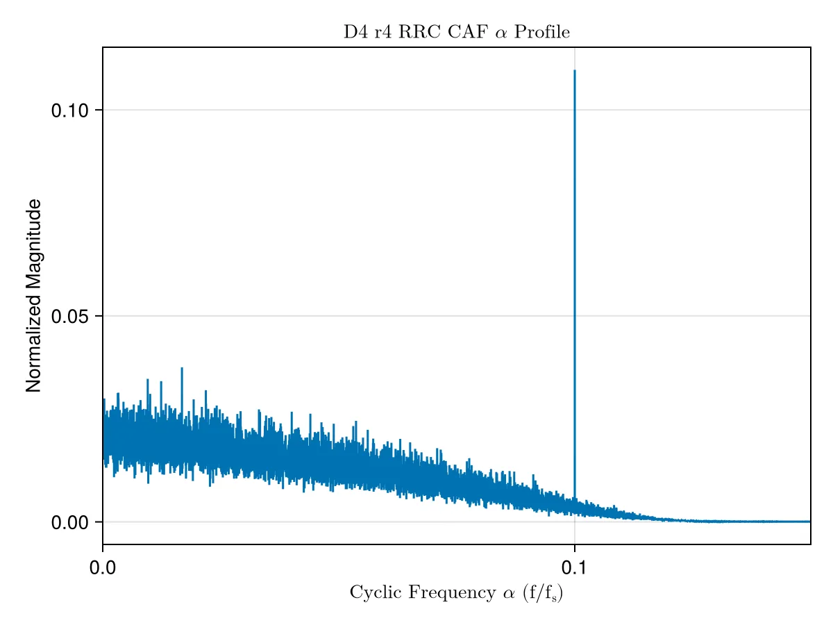
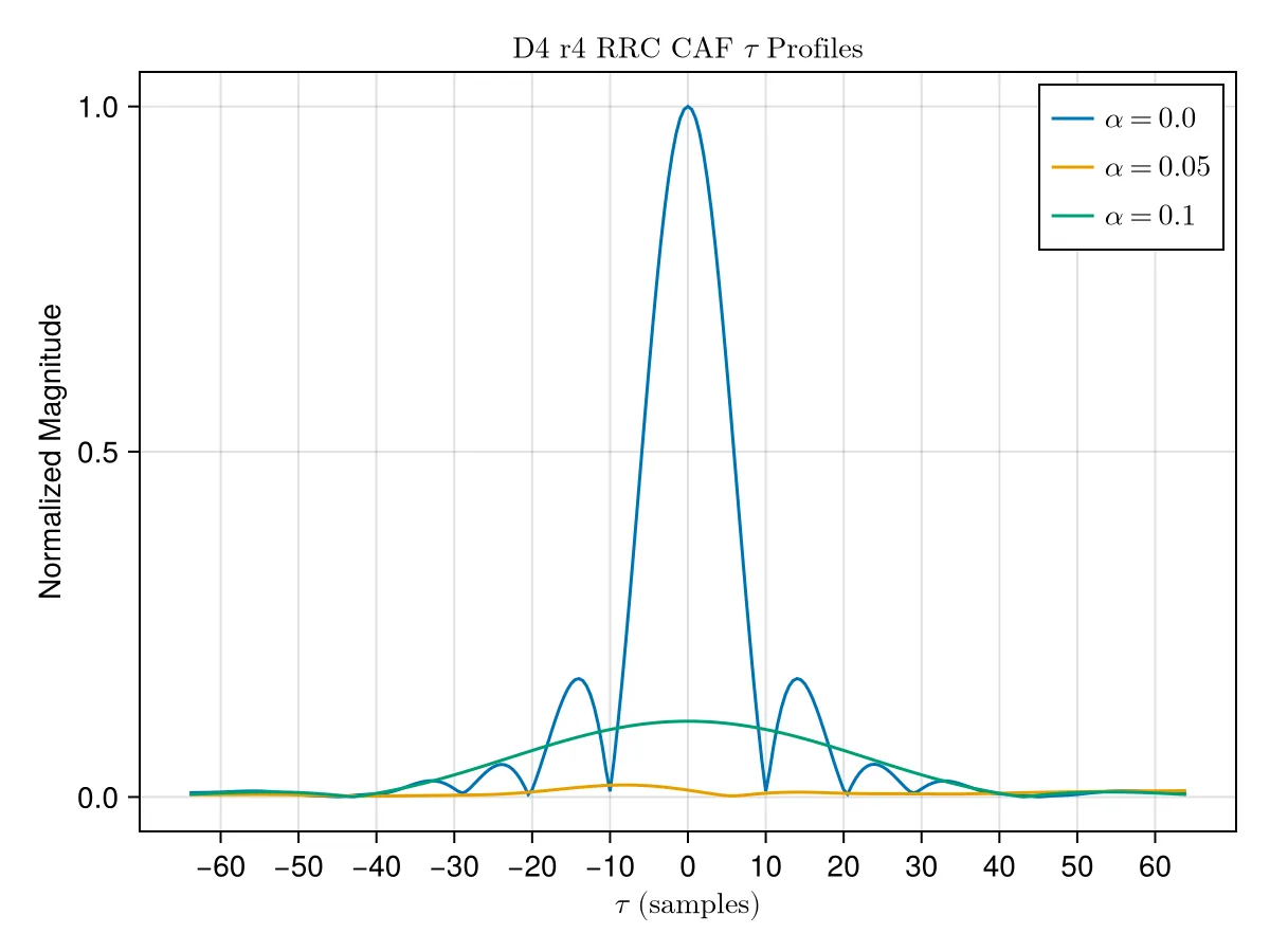
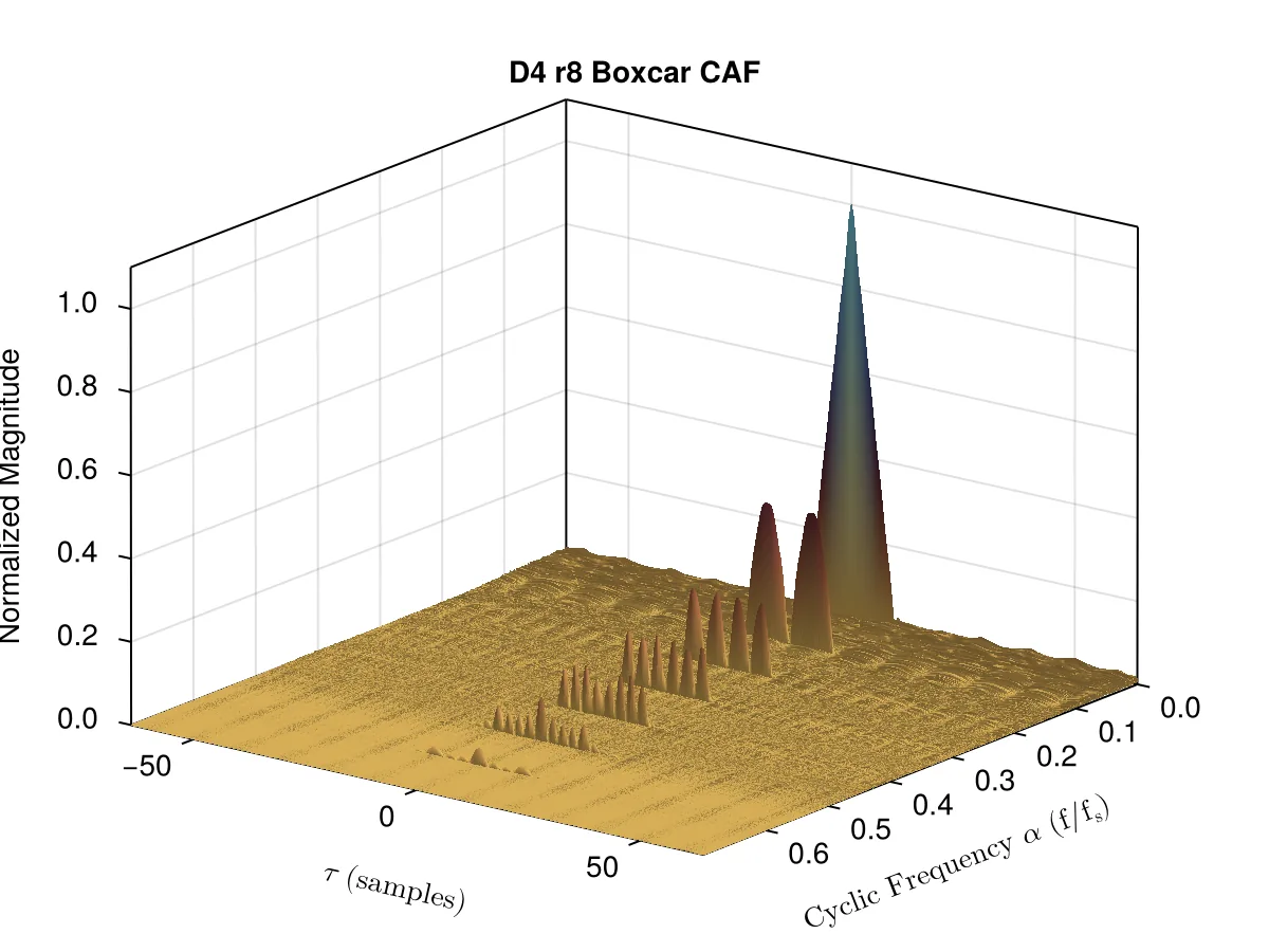
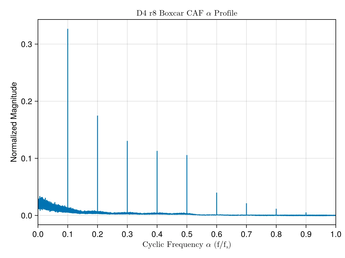
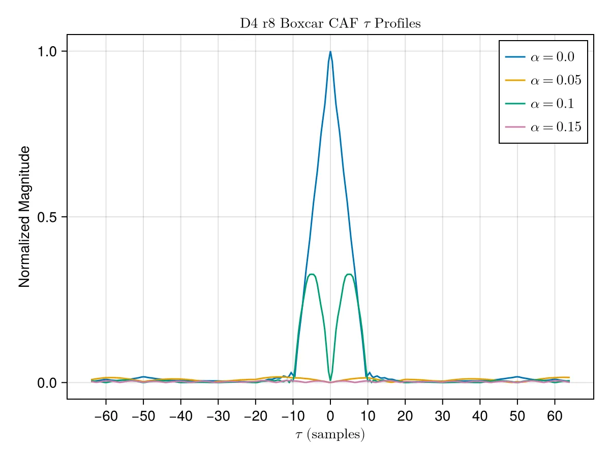
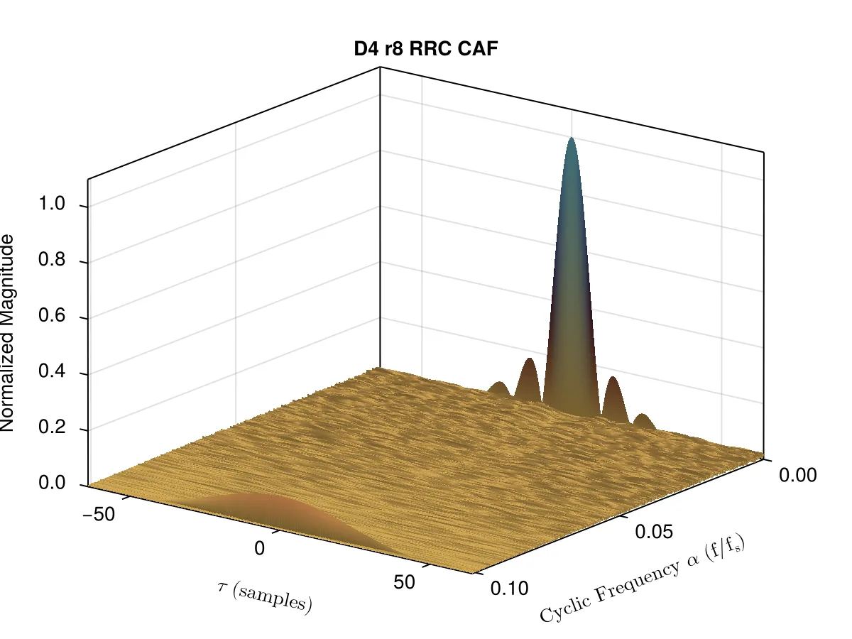
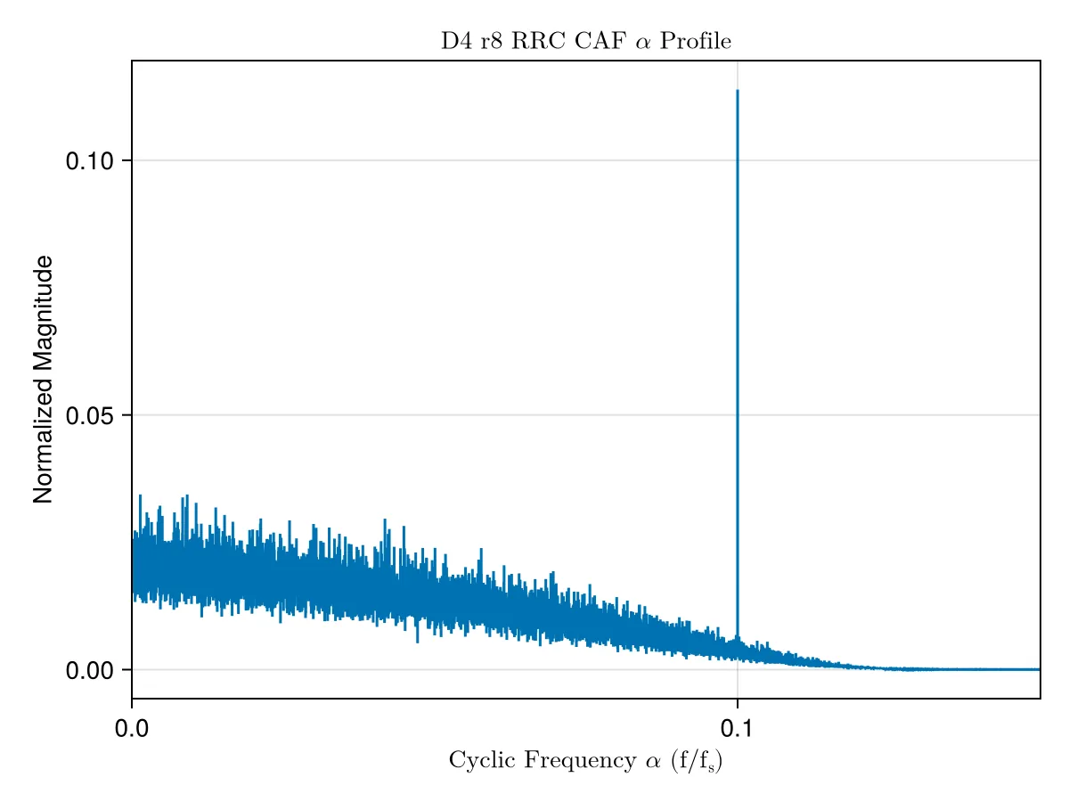
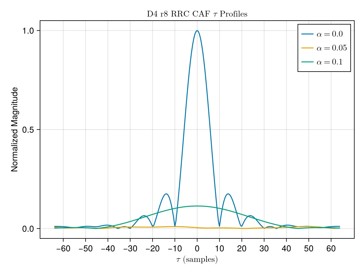
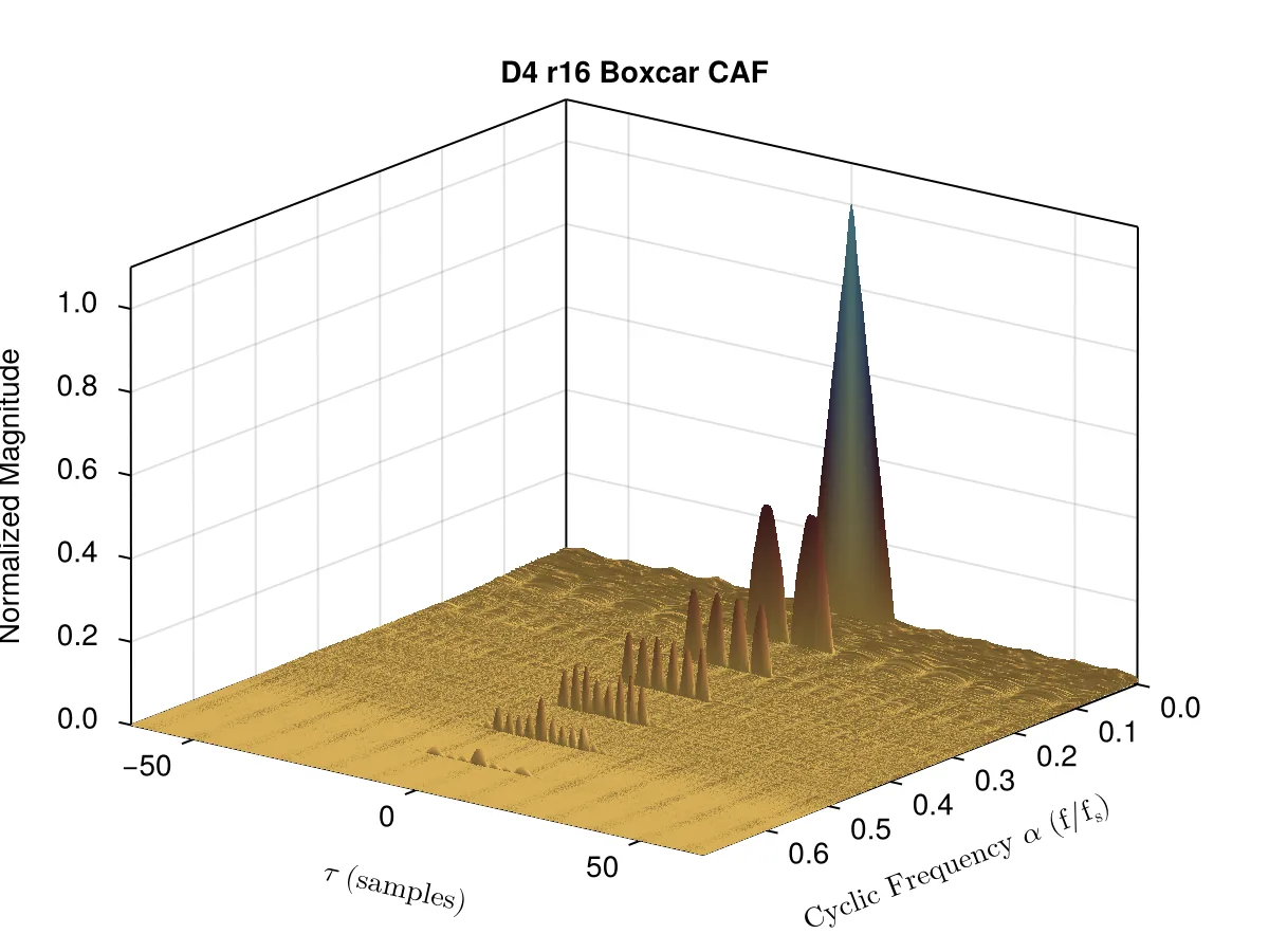
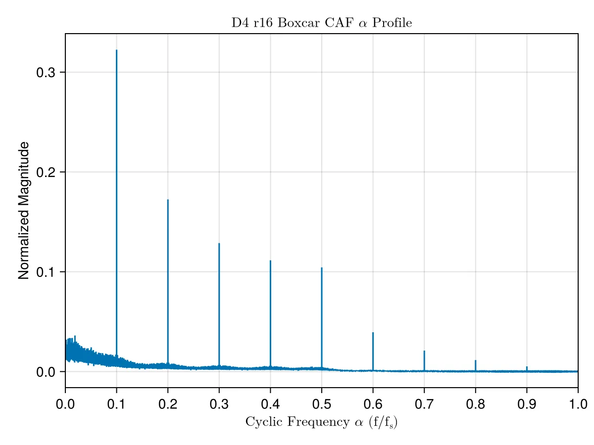
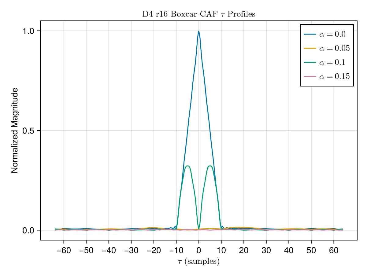
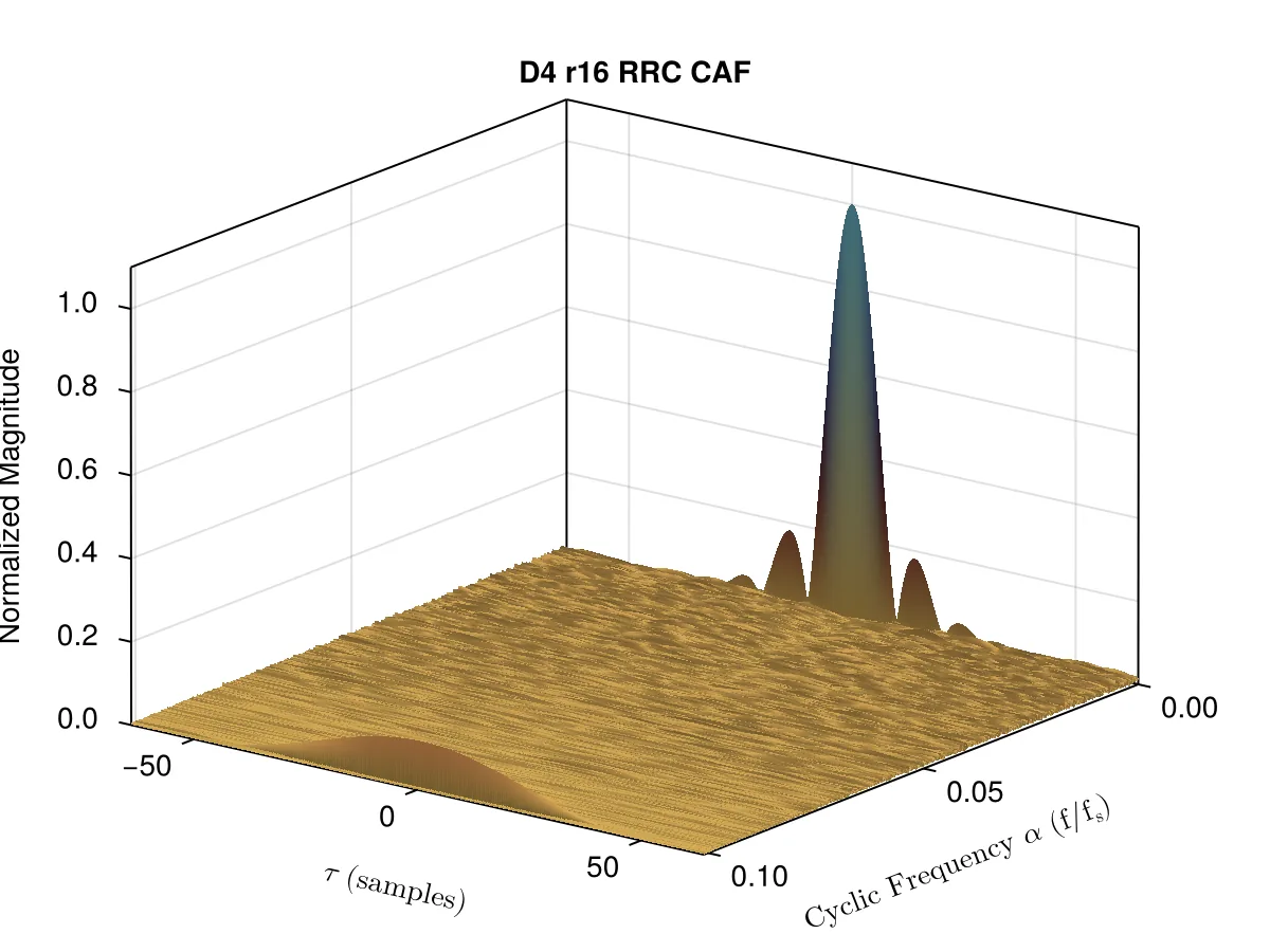
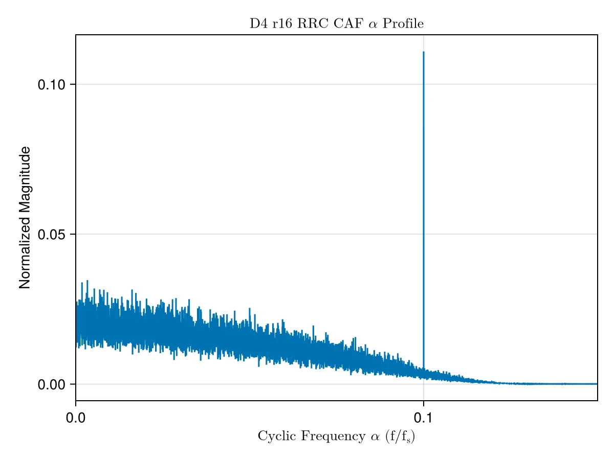
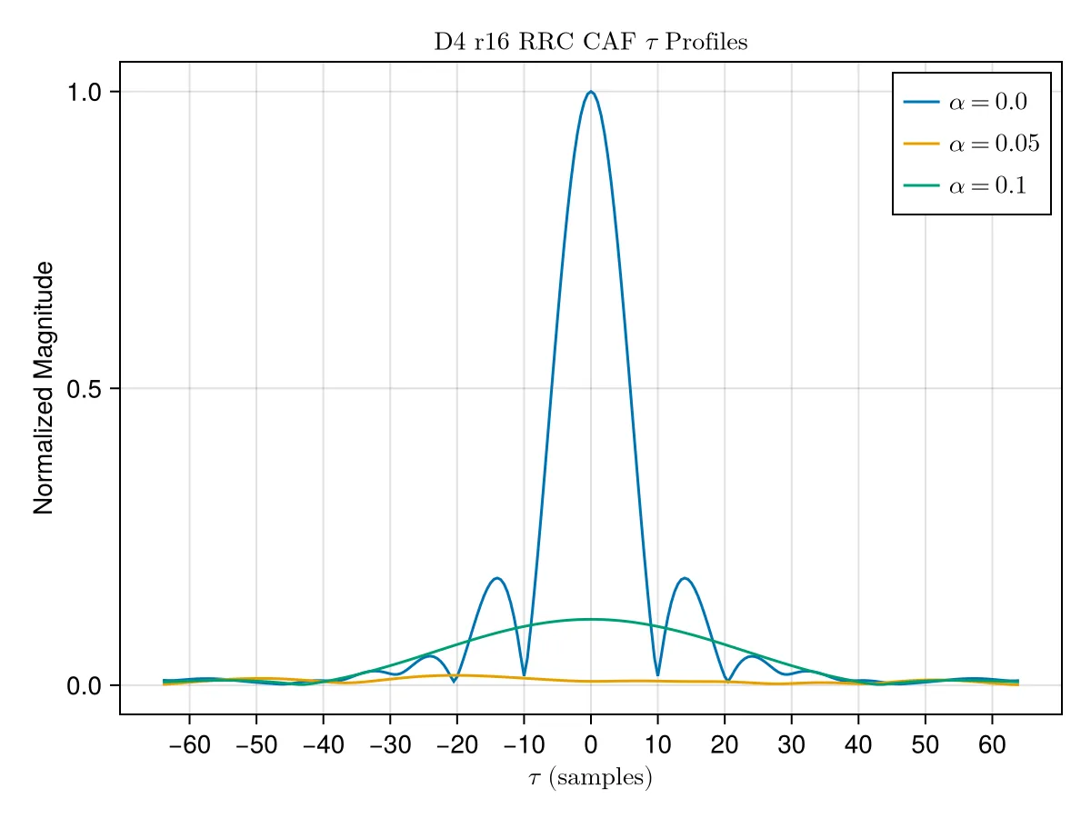
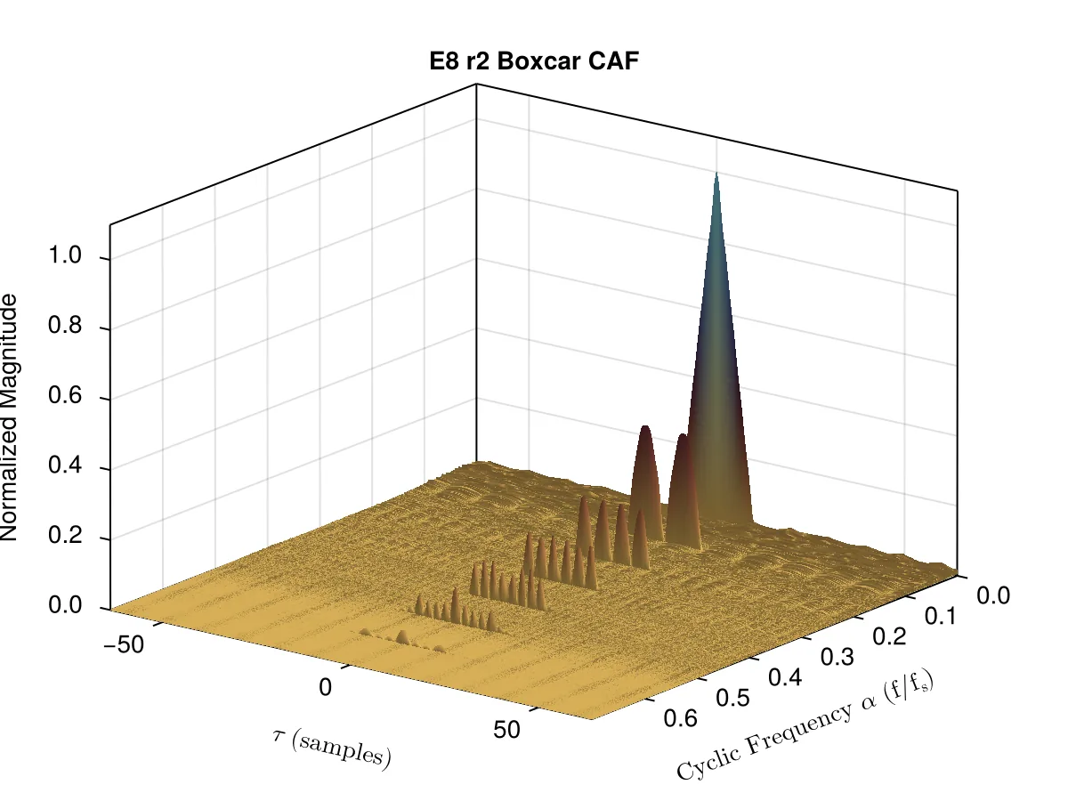
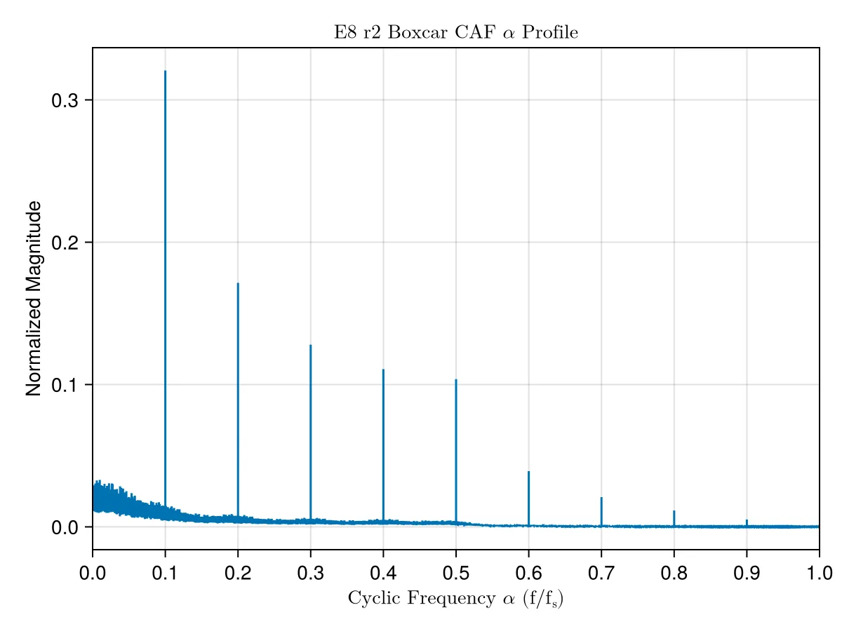
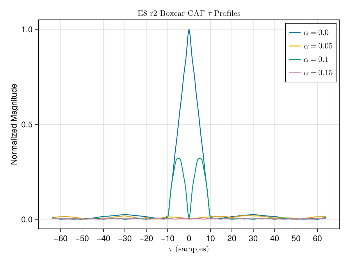
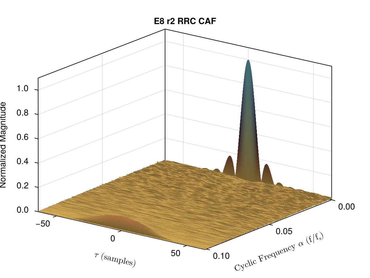
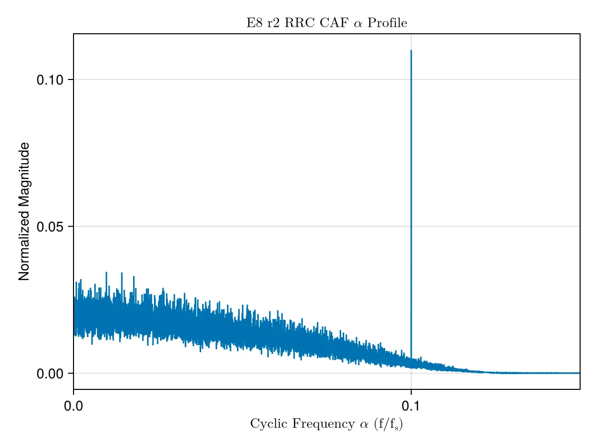
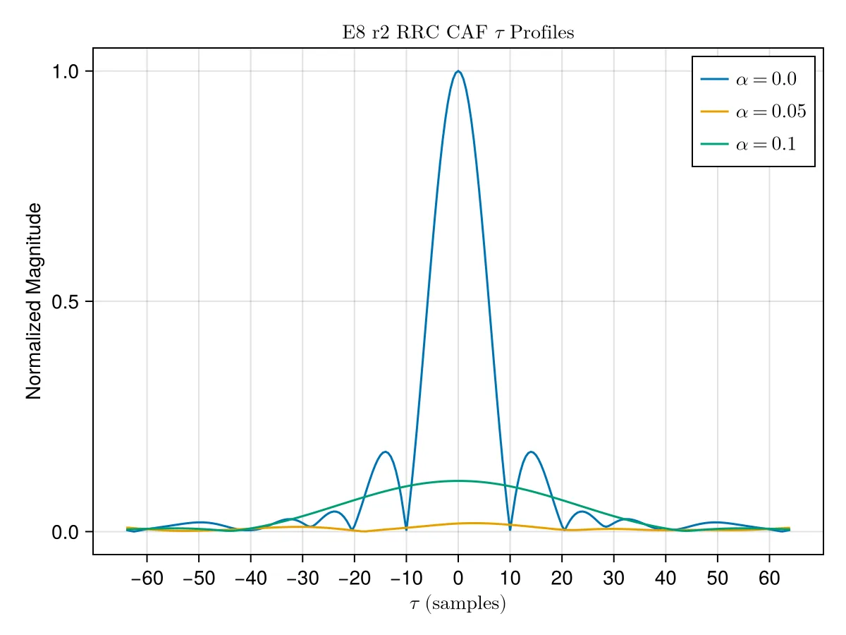
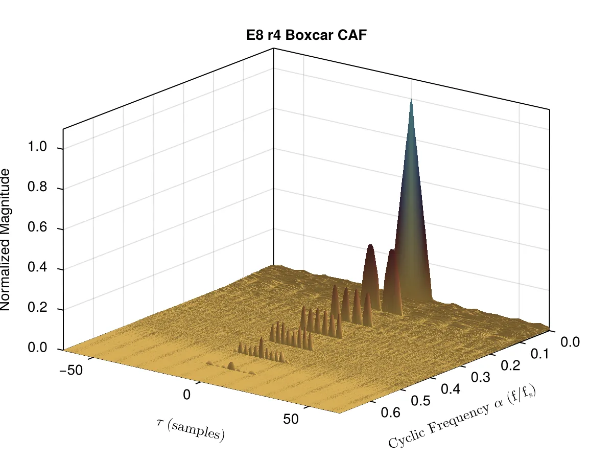
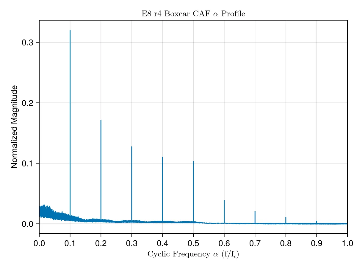
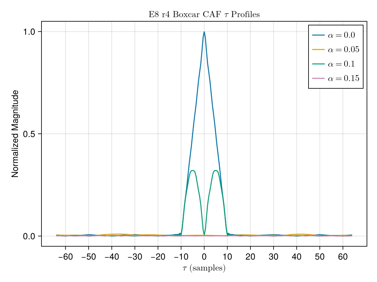
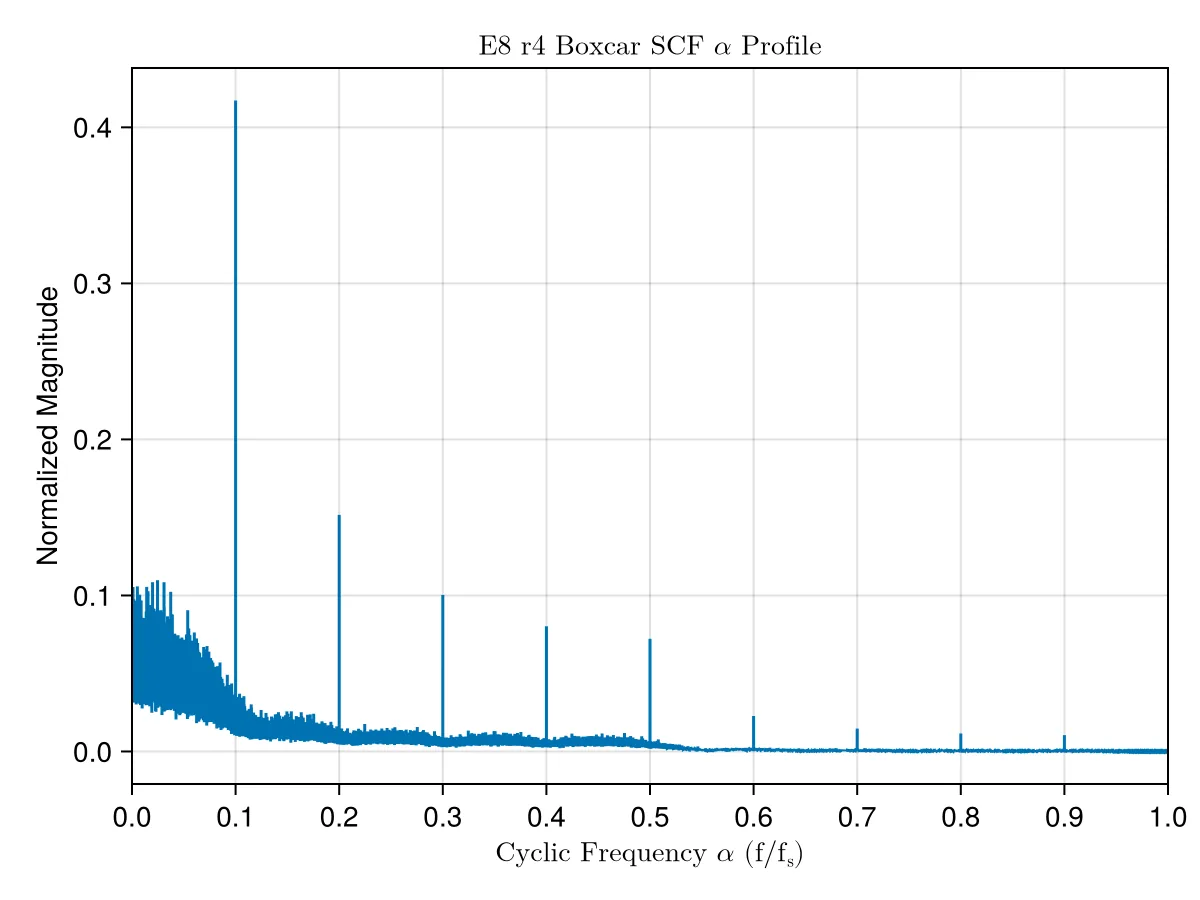
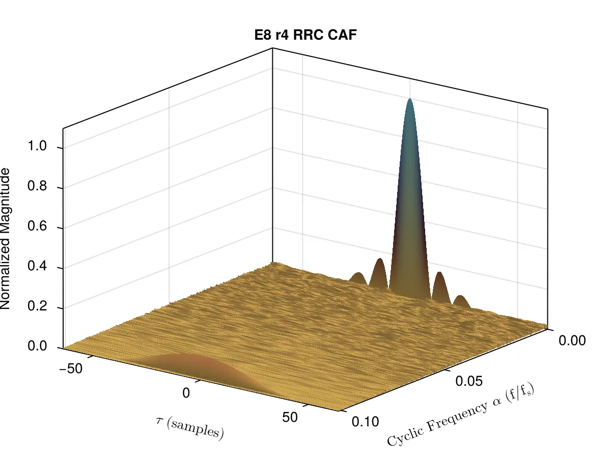
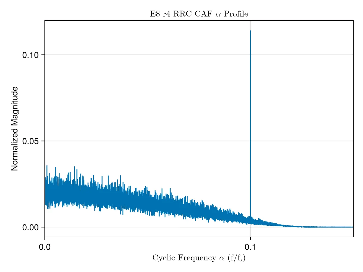
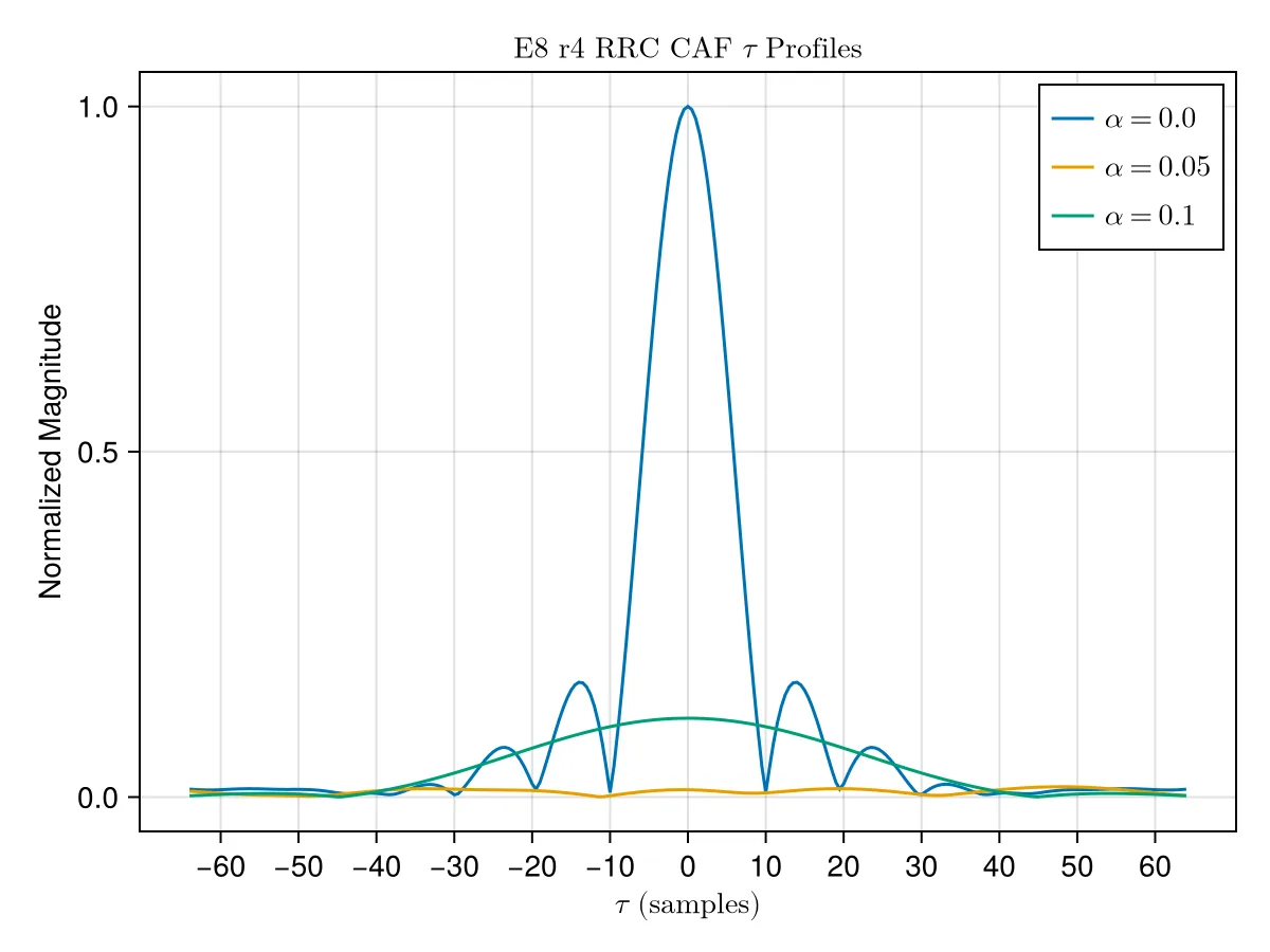
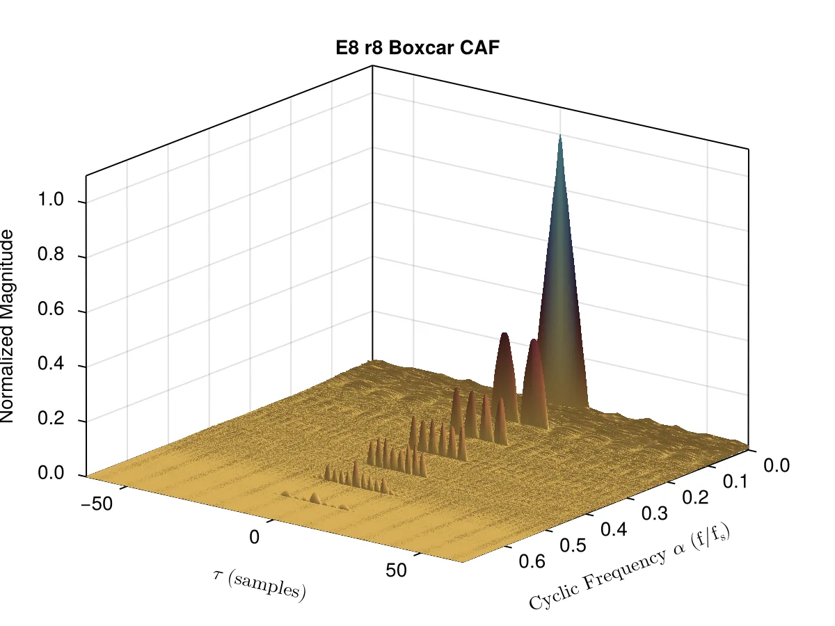
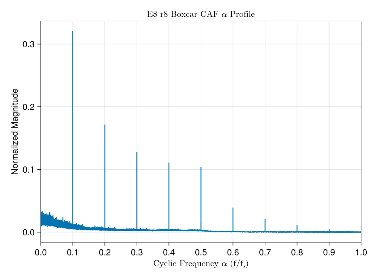
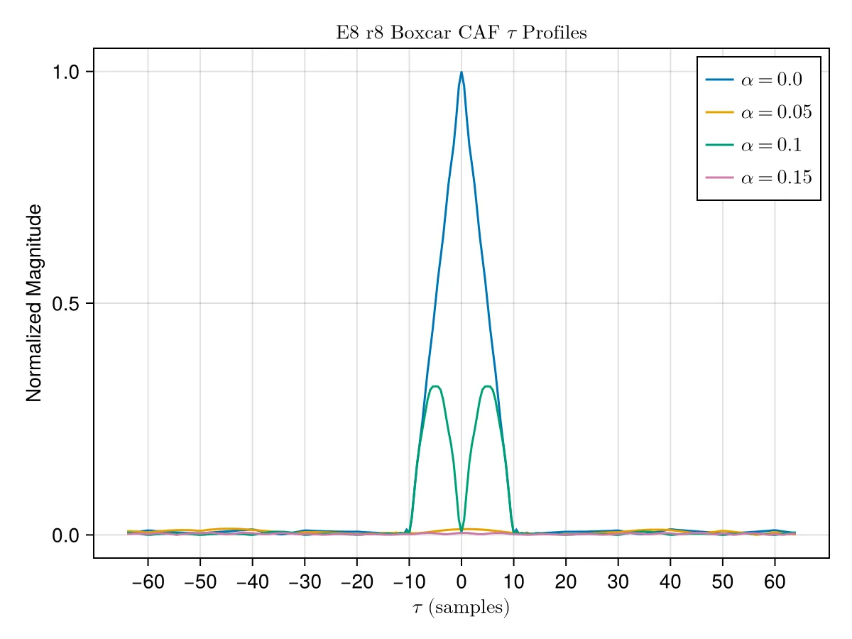
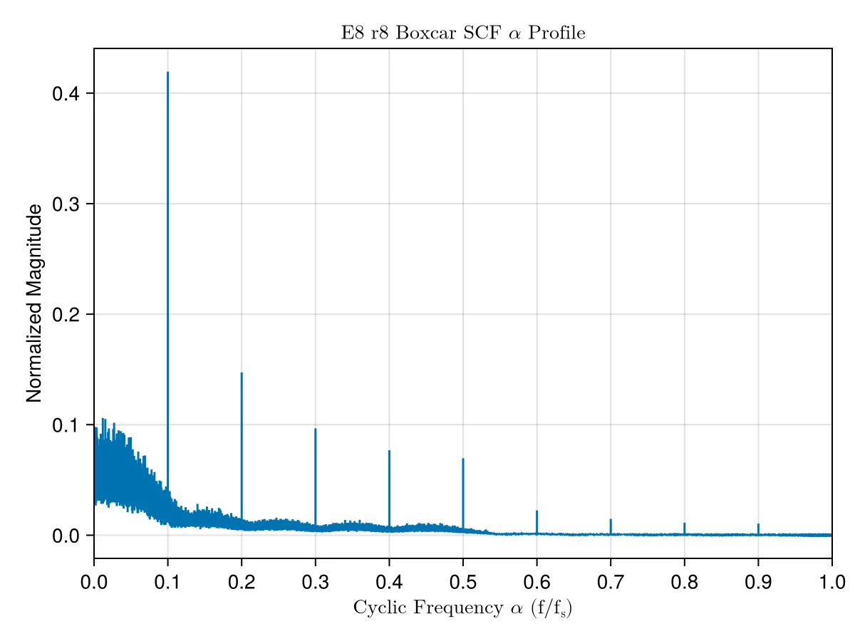
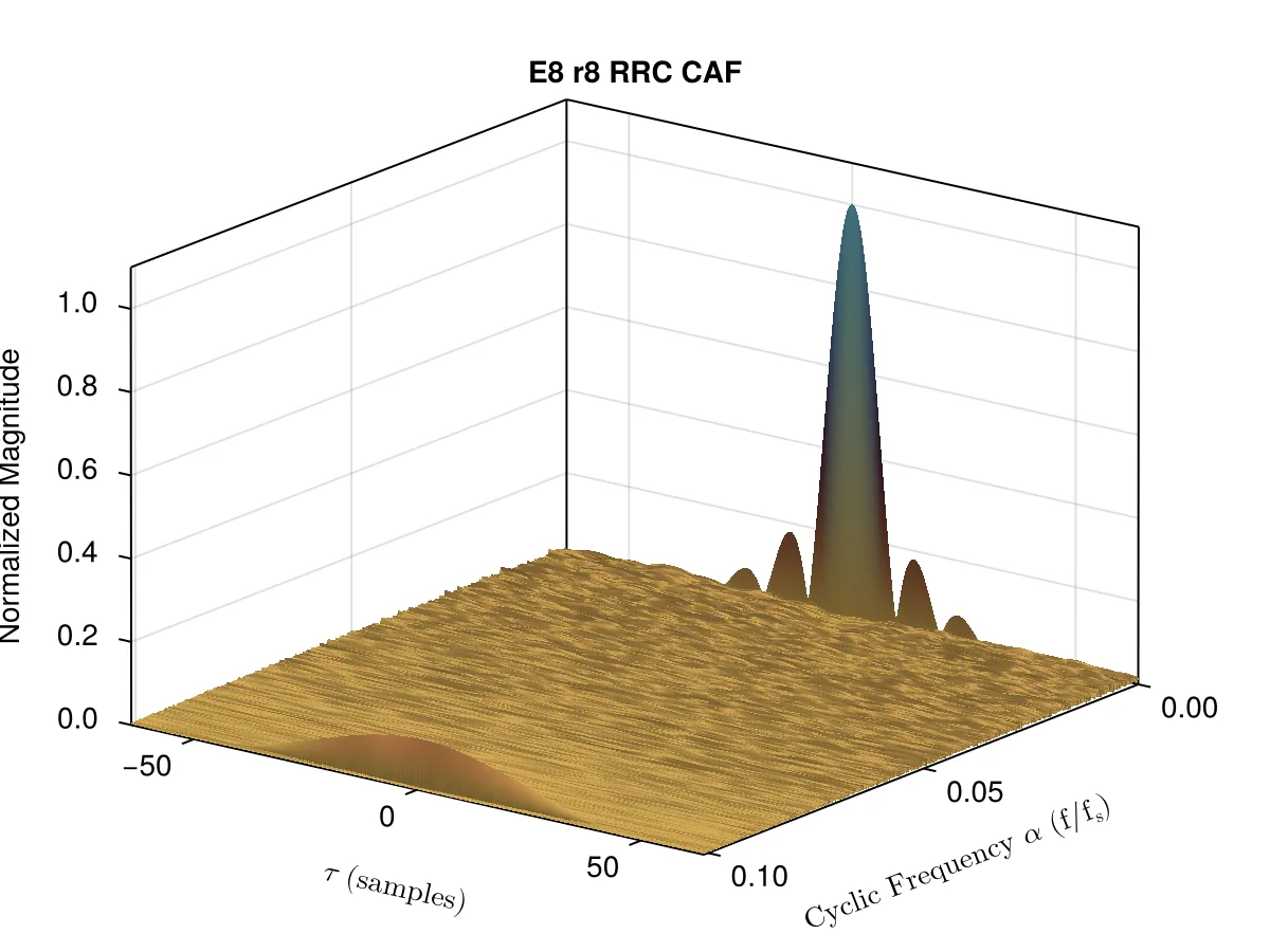
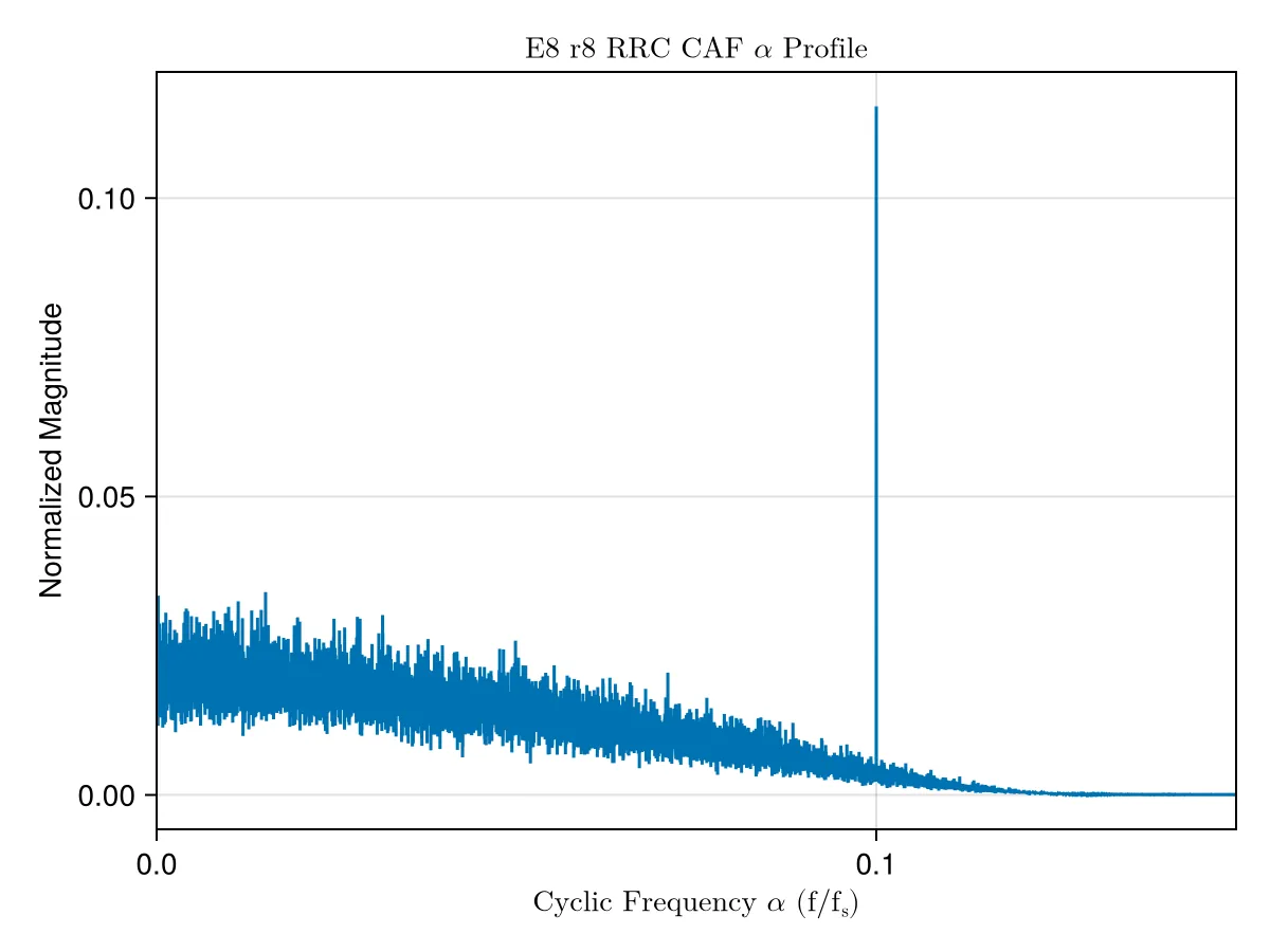
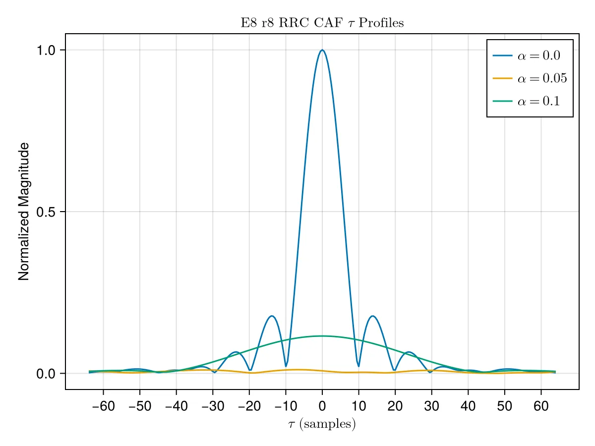
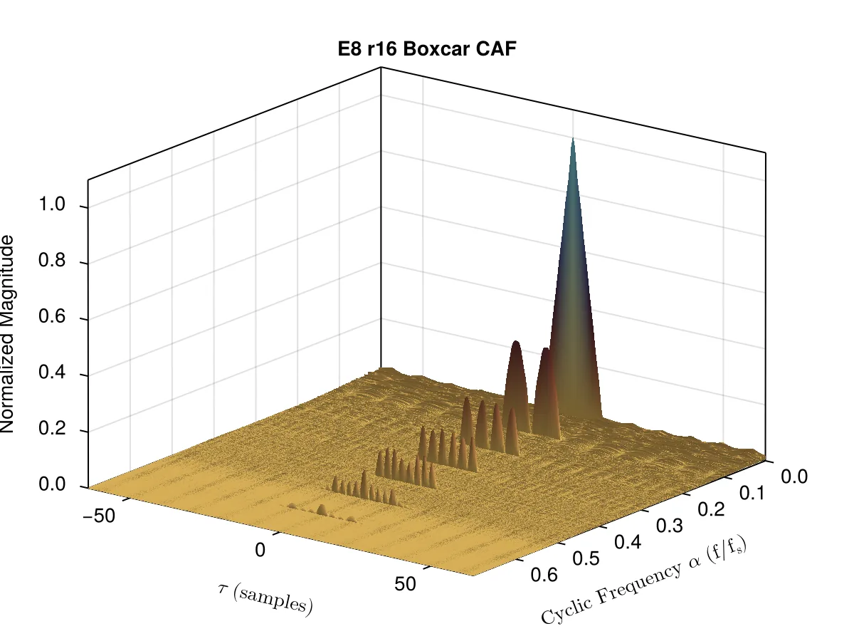
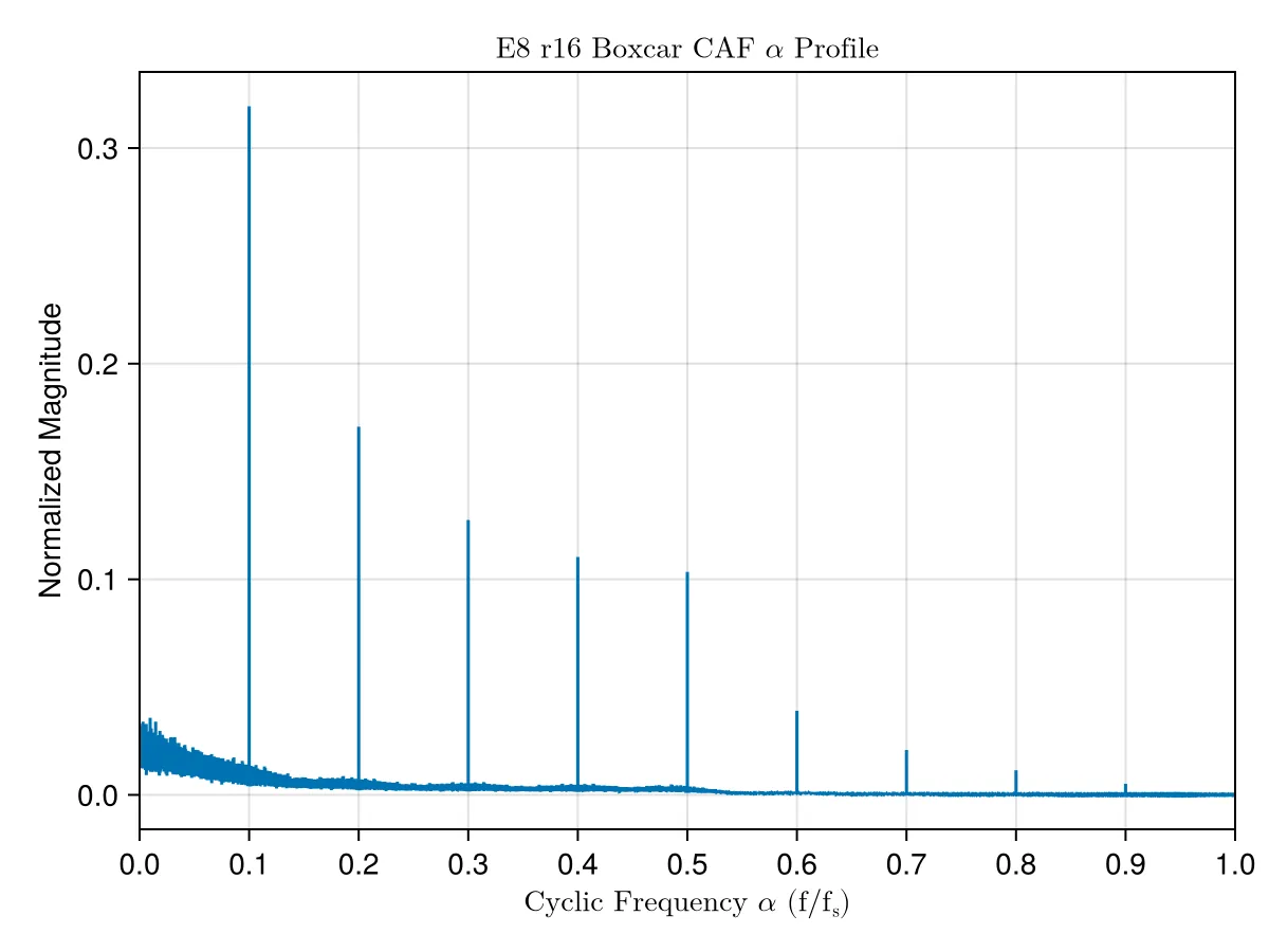
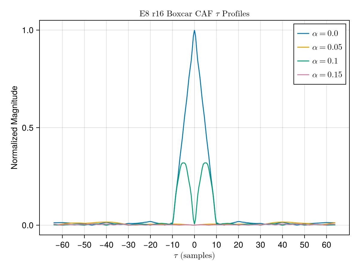
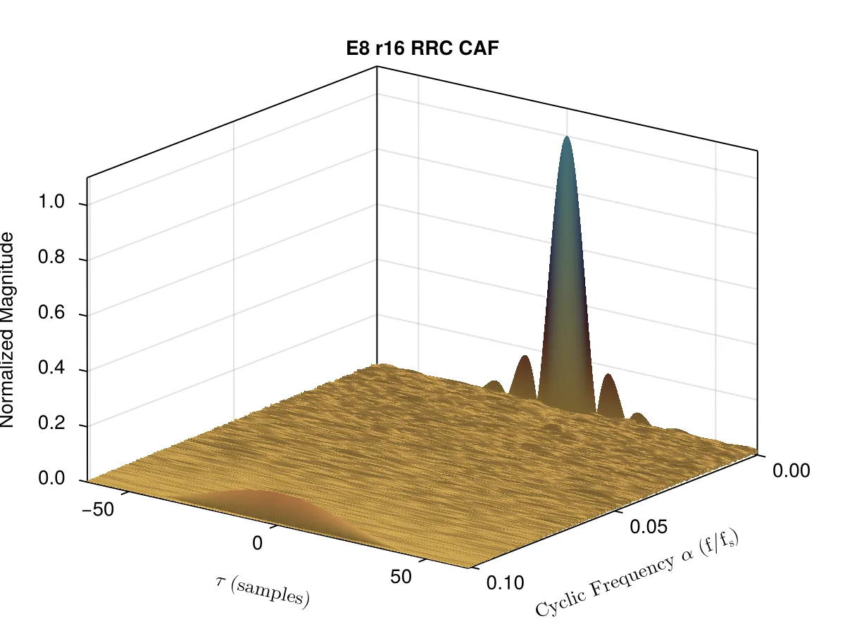
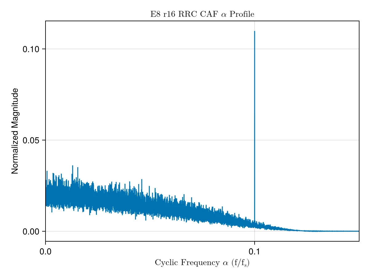
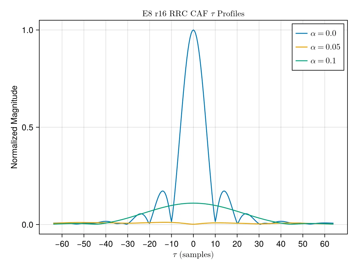
The CAF plot identifies the repetitive structure of a signal’s power over time, like symbol rate. Here, variable alpha represents the cyclic frequency and tau represents the lag product. When a boxcar filter is used, the tau-profiles spike like rows of teeth. When an RRC filter is used, the tau-profile resembles a sinc function. For a signal upsampled by x, the CAF plot shows spikes for alpha values related to 1/x. The boxcar filter will show repeated spikes at alpha = n/x, n ∈ {0, 1, 2, 3, …, x – 1} with the magnitude decreasing as n increases,while the RRC filter will only show at 0 and 1/x. Likewise, this symbol rate can be seen in the alpha = 0 tau-profile, where the base of the peak is -/+ x. For these plots, the signal is upsampled by 10, so we see spikes in the alpha profile at alpha = 1/10, 2/10, 3/10, etc. We also see in the alpha = 0 tau-profiles, the base of the peak for both filters corresponds to -/+ 10.

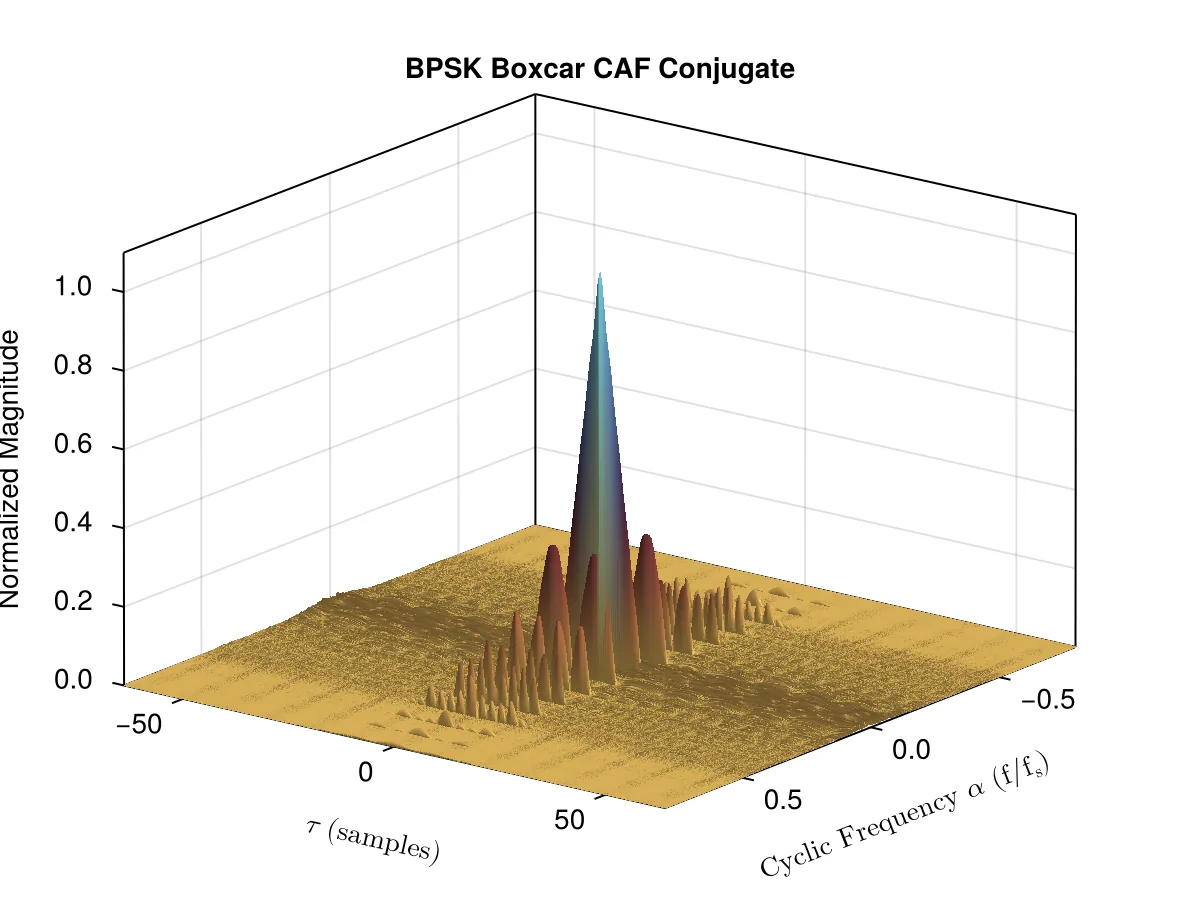
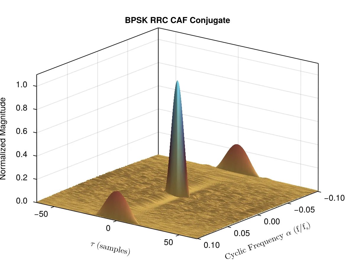
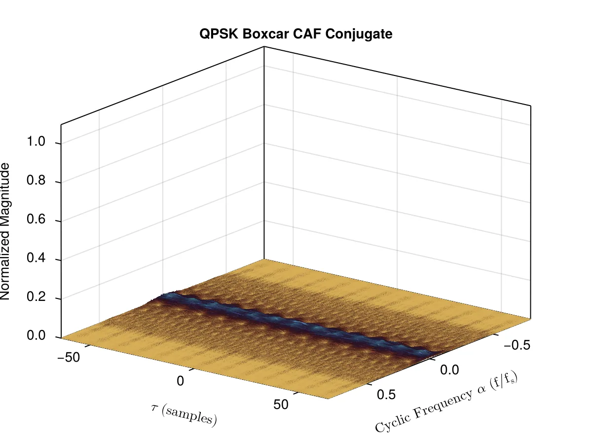
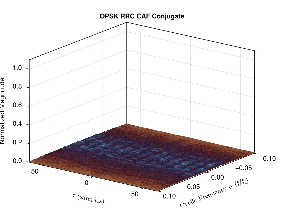
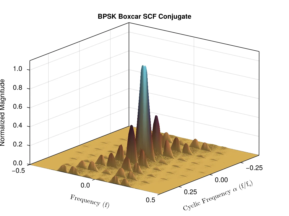
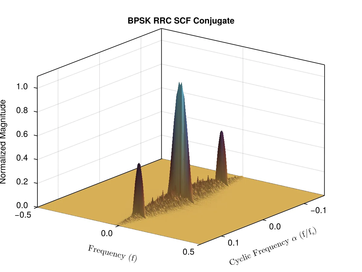
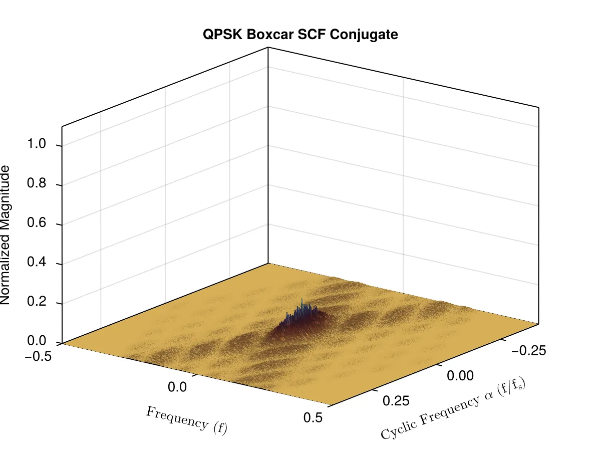
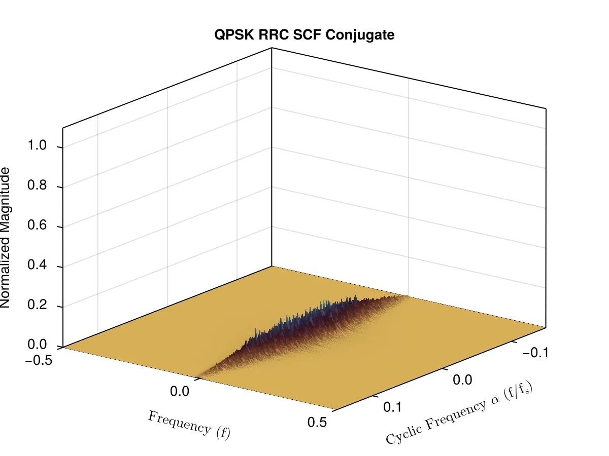
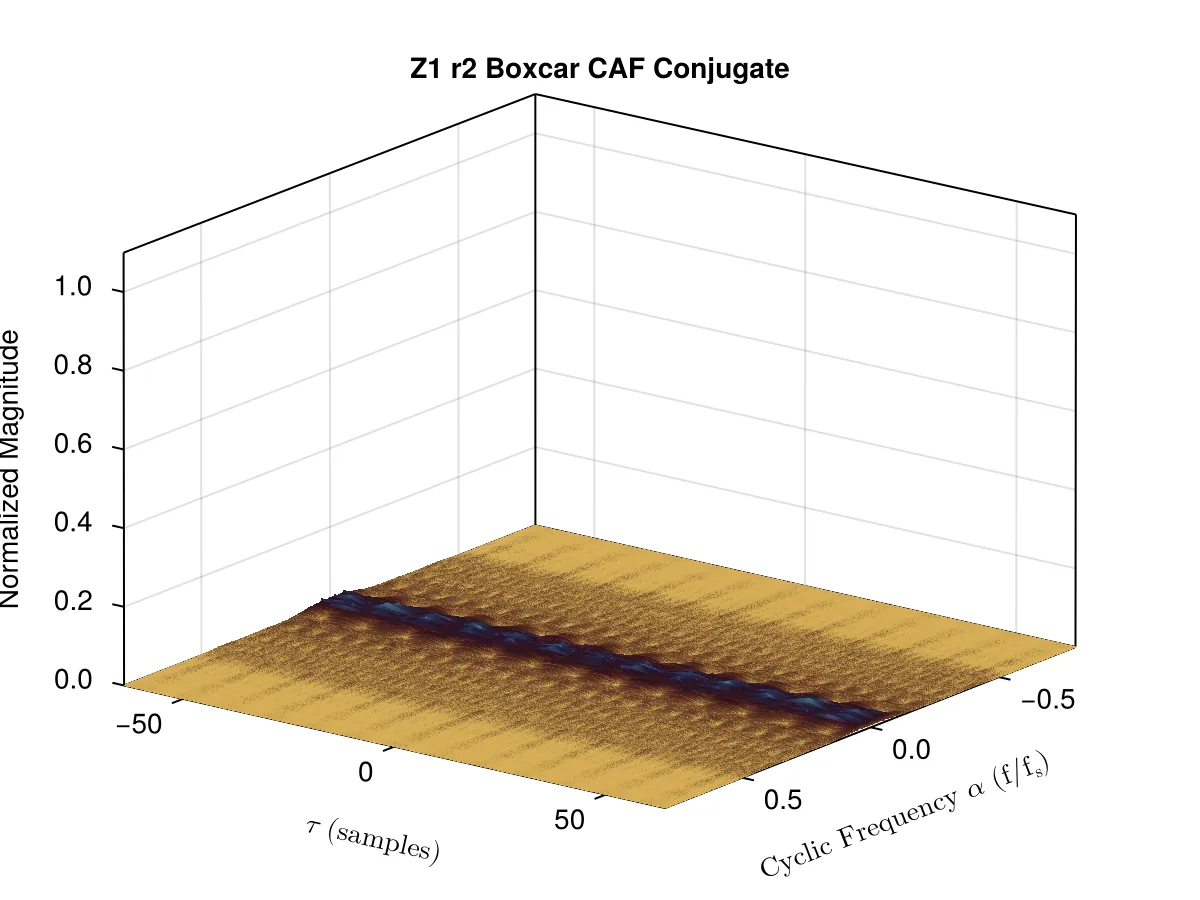
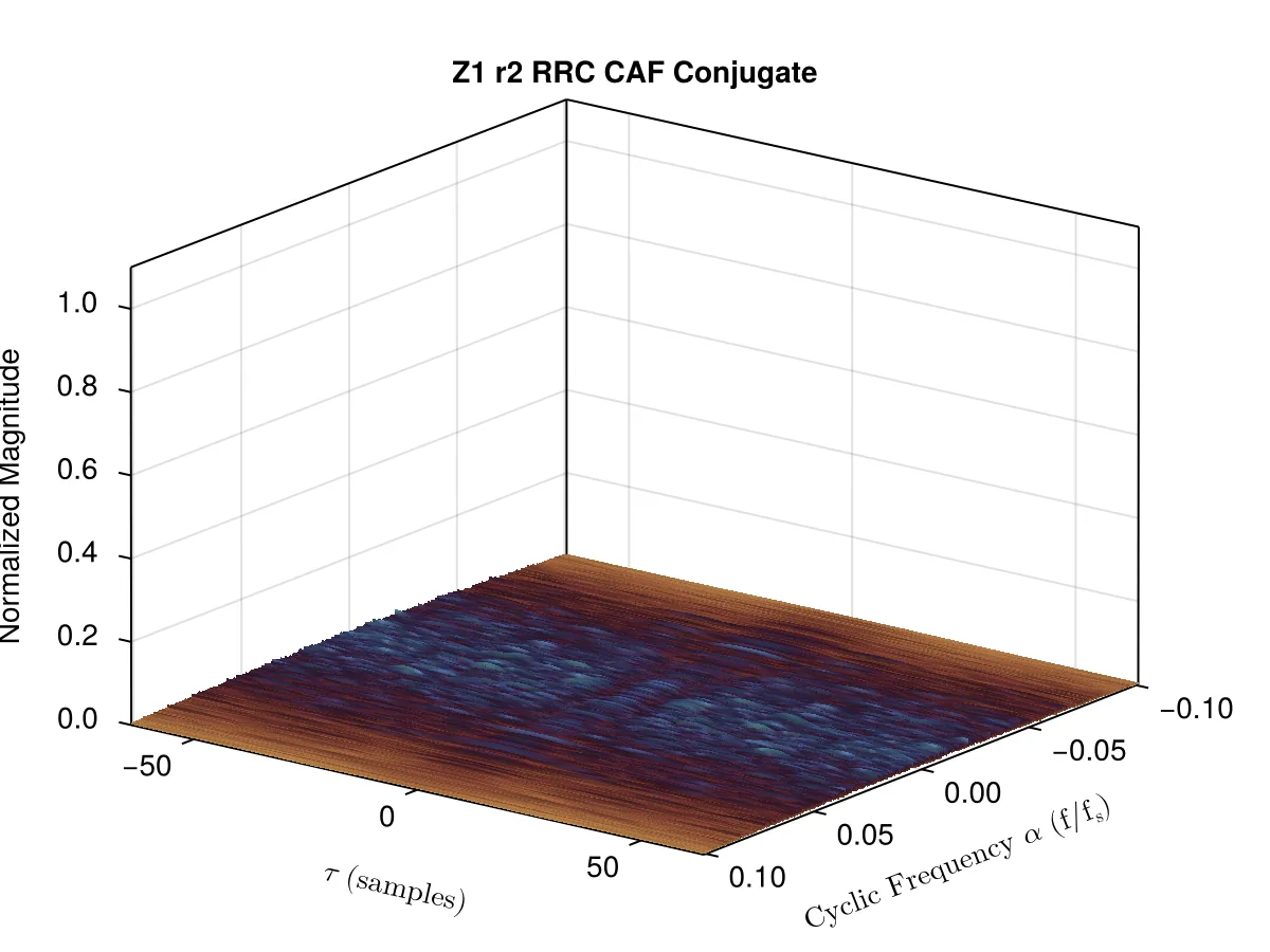
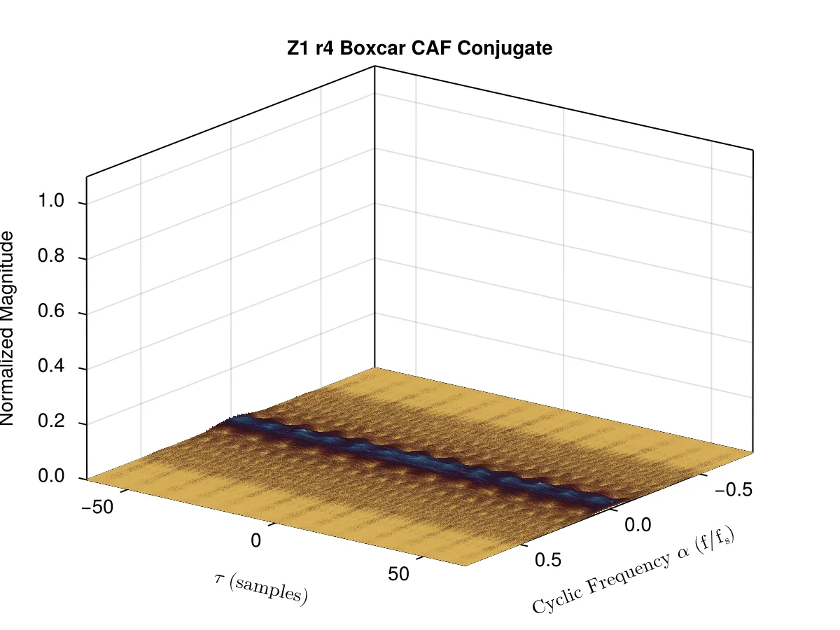
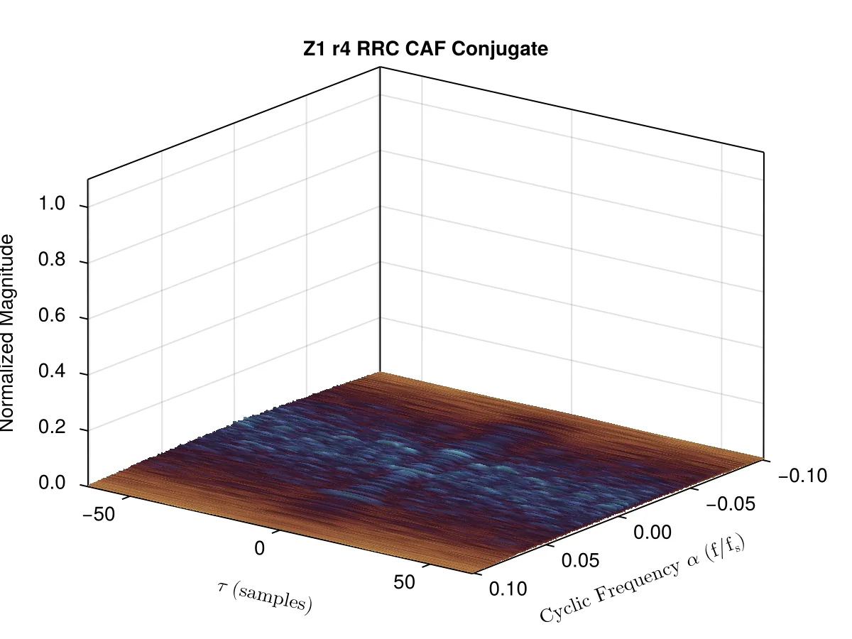
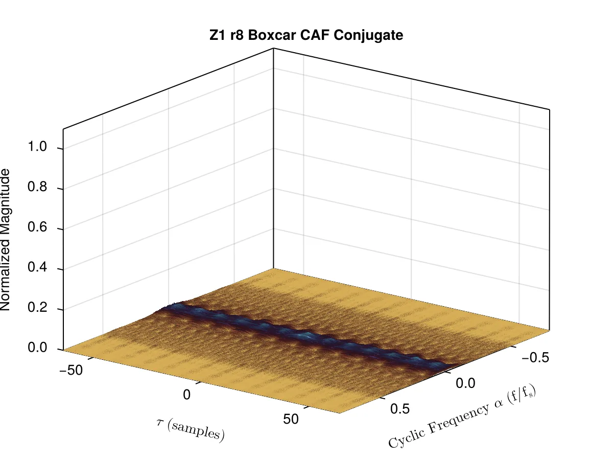
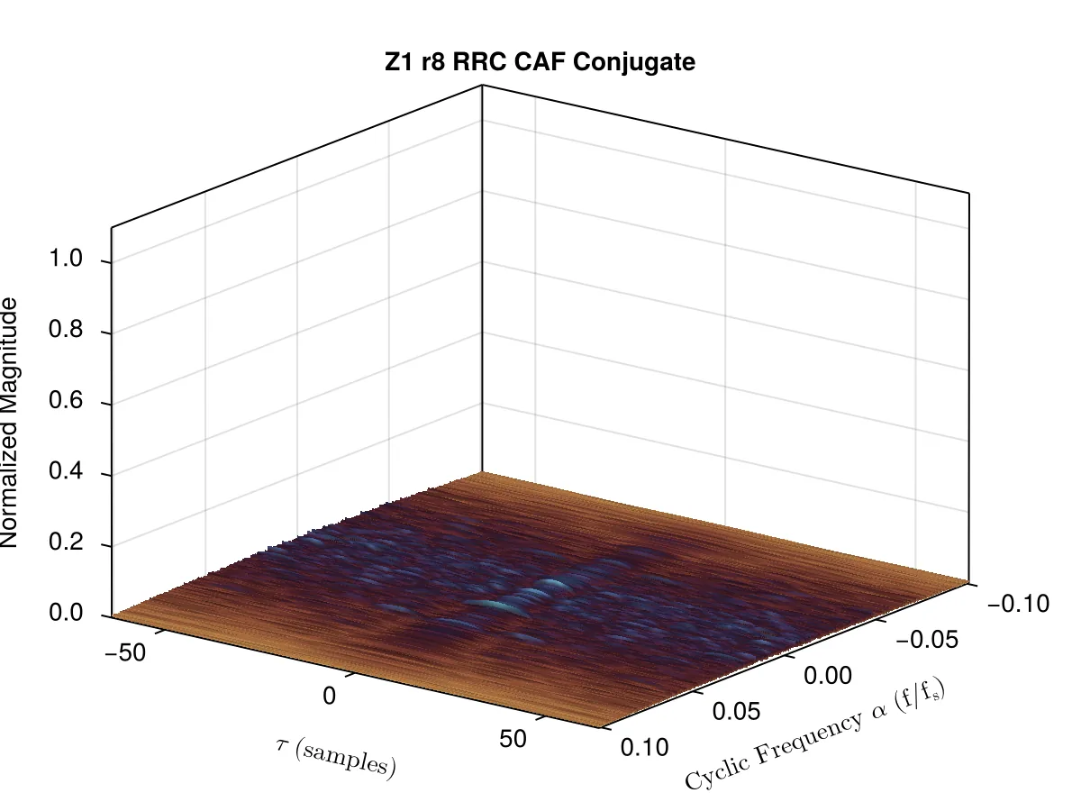
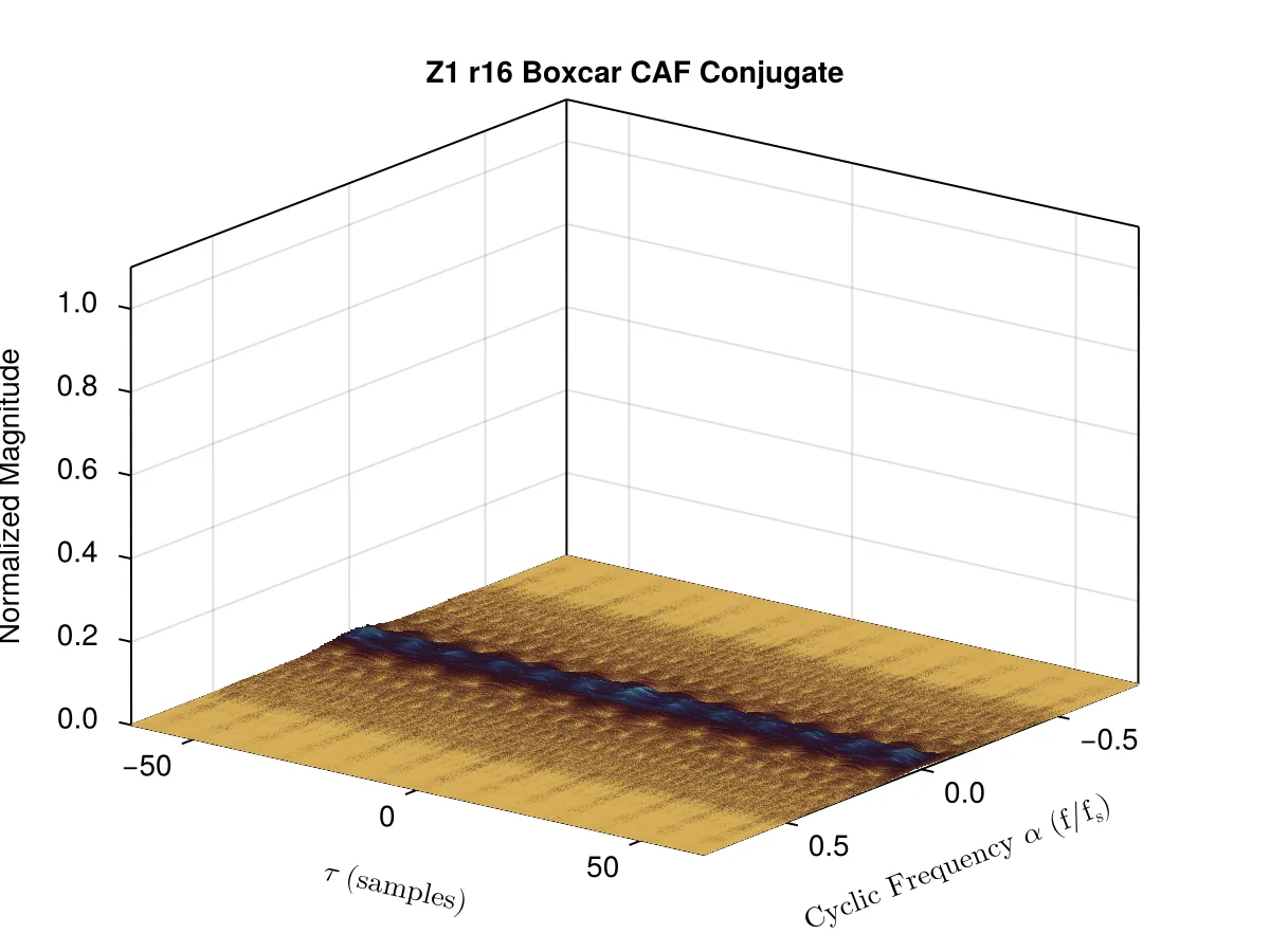
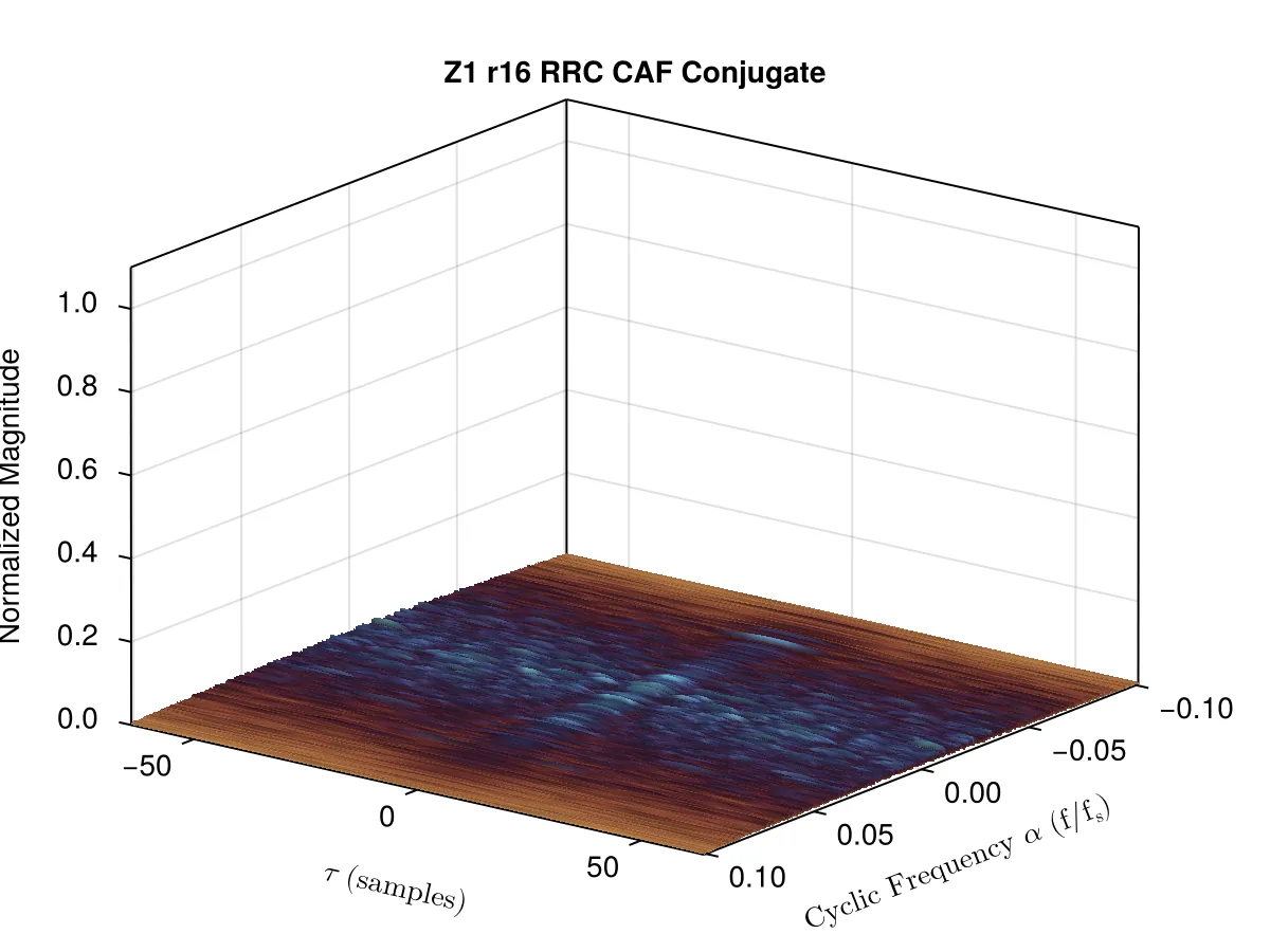
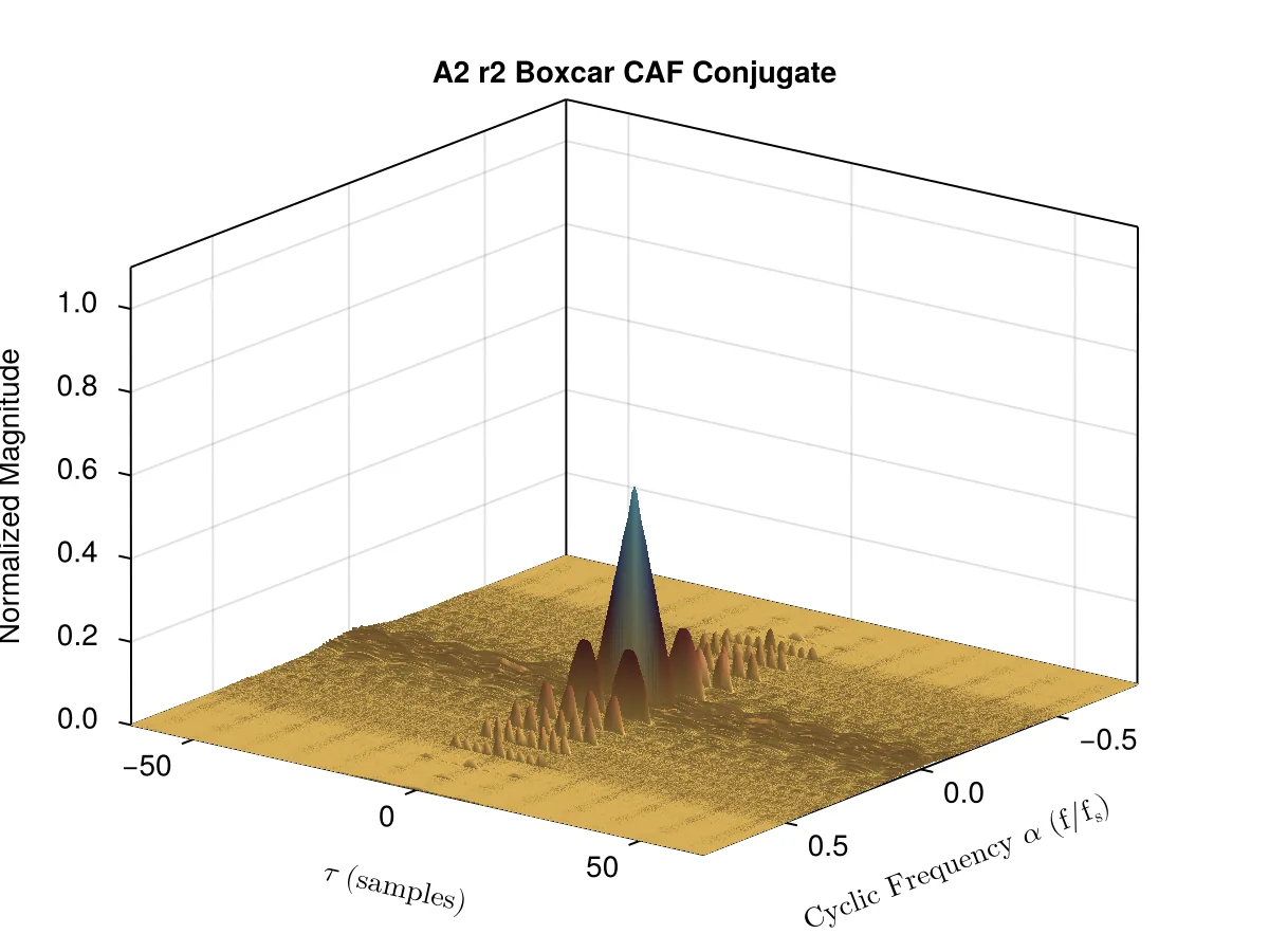
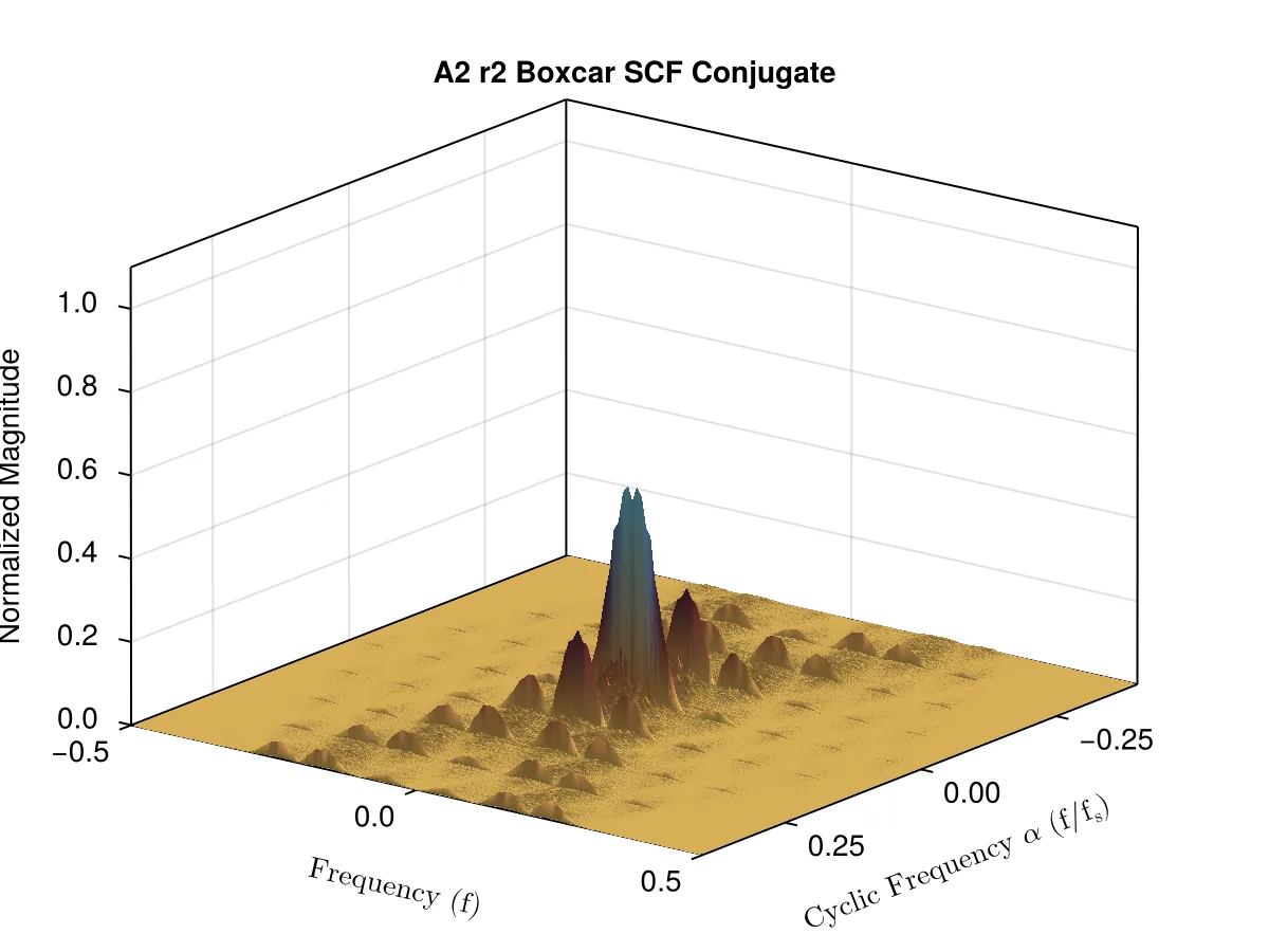
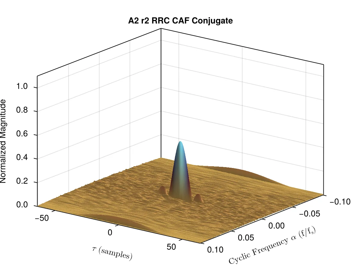
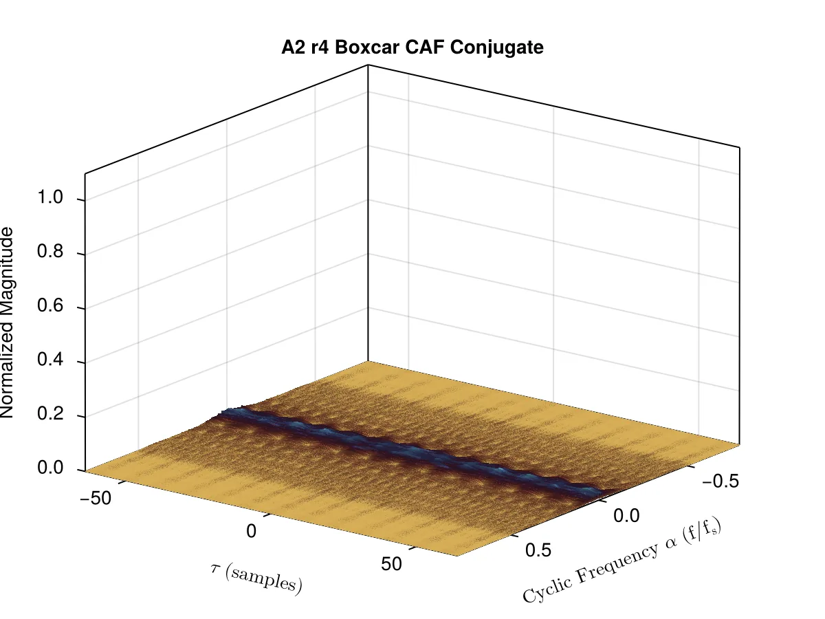
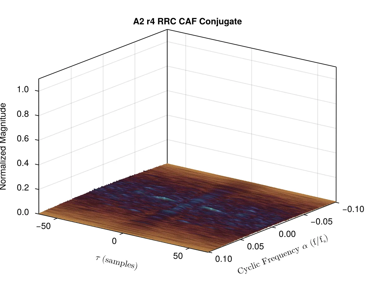
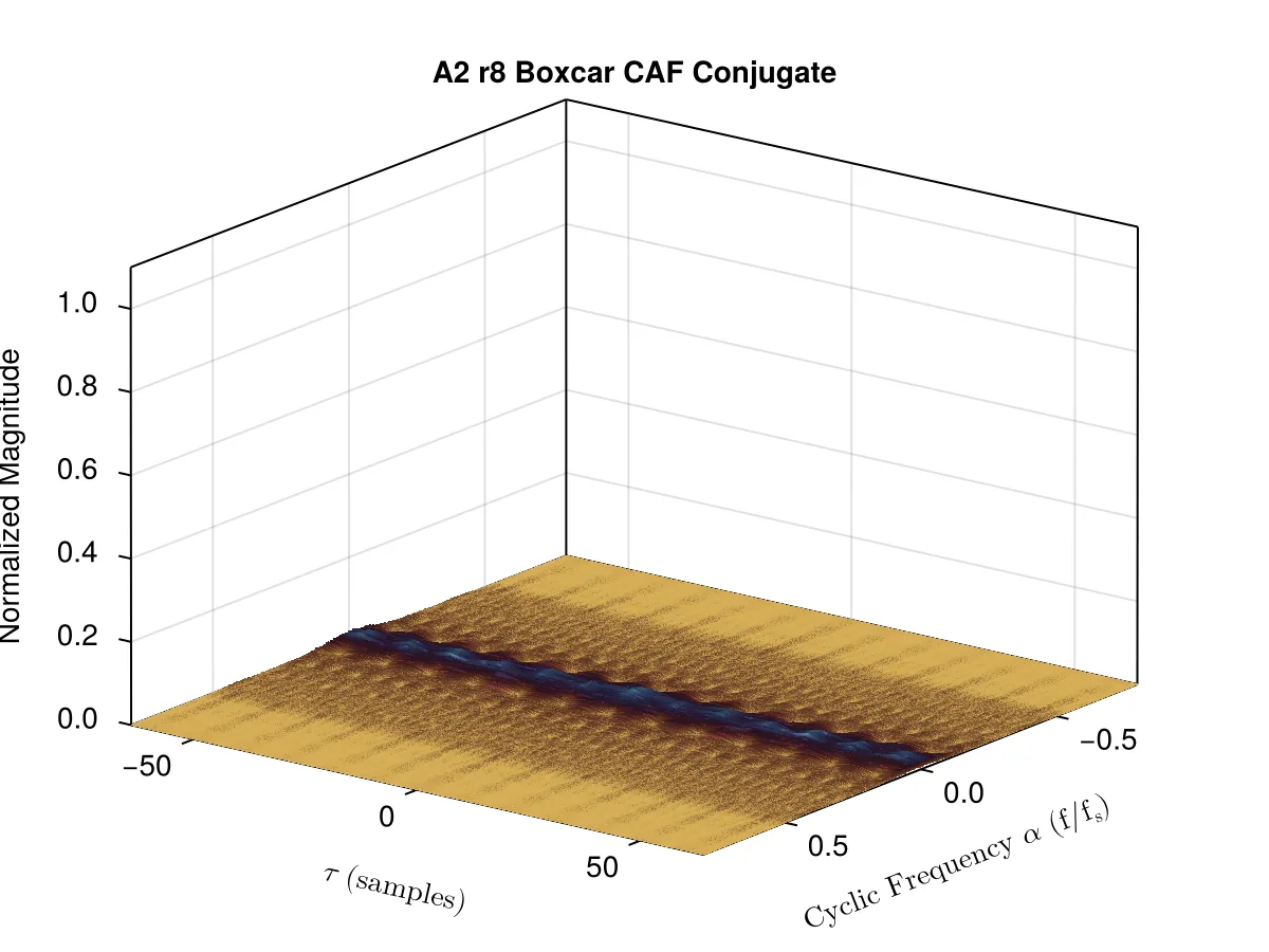
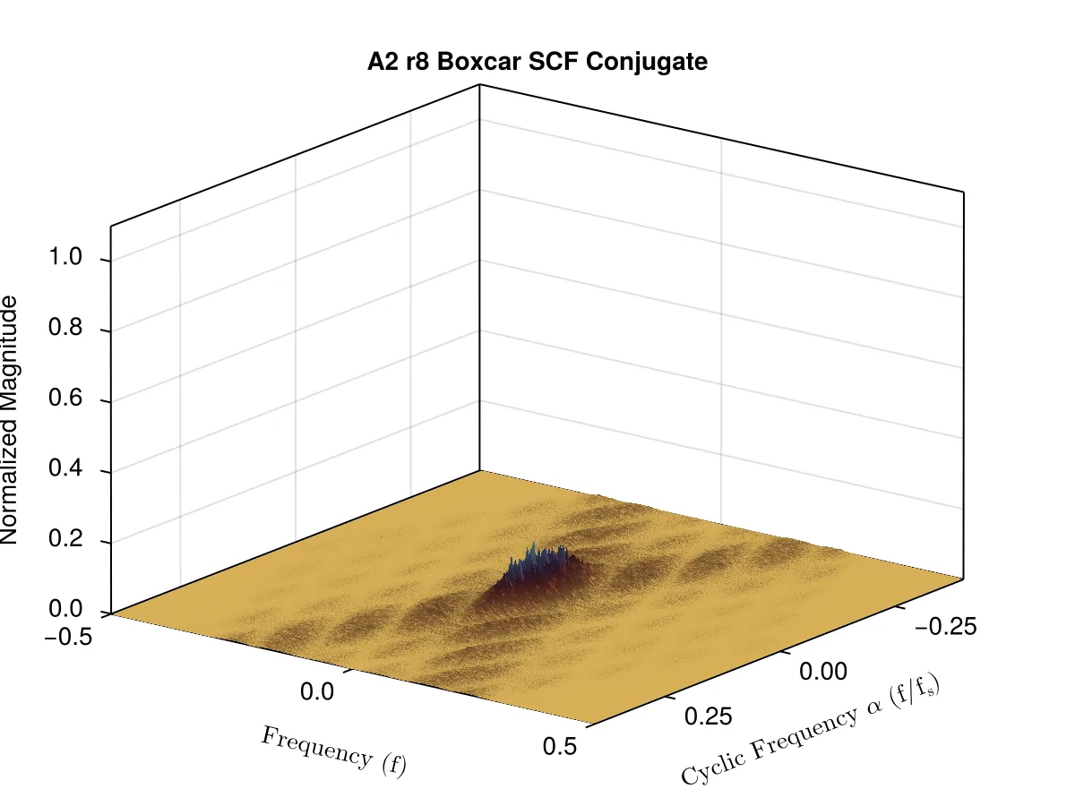
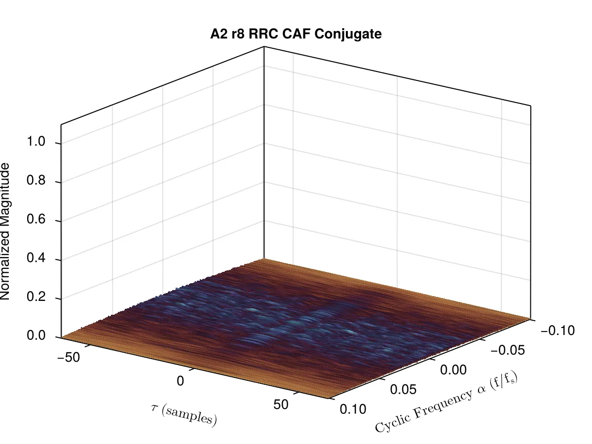
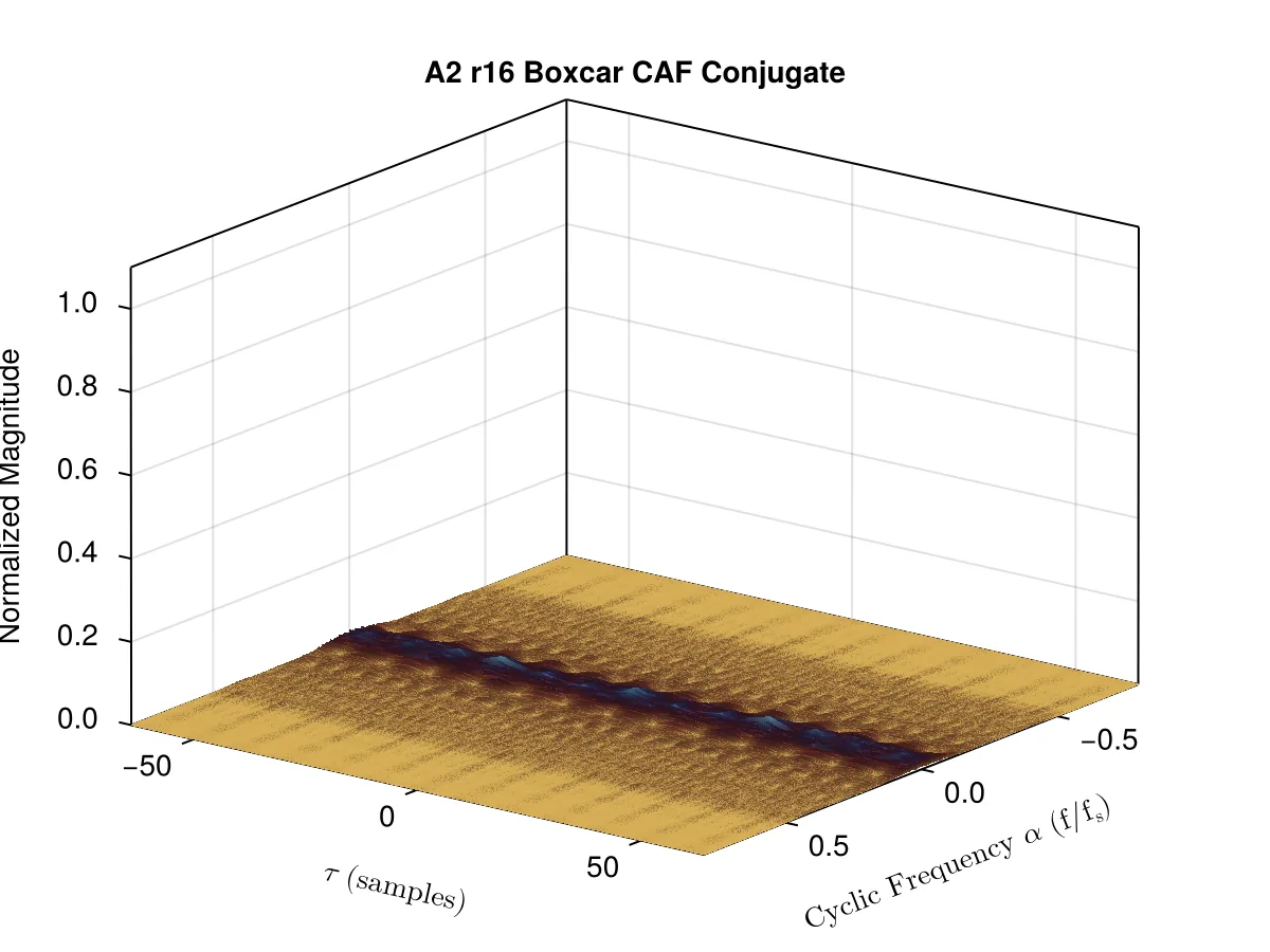
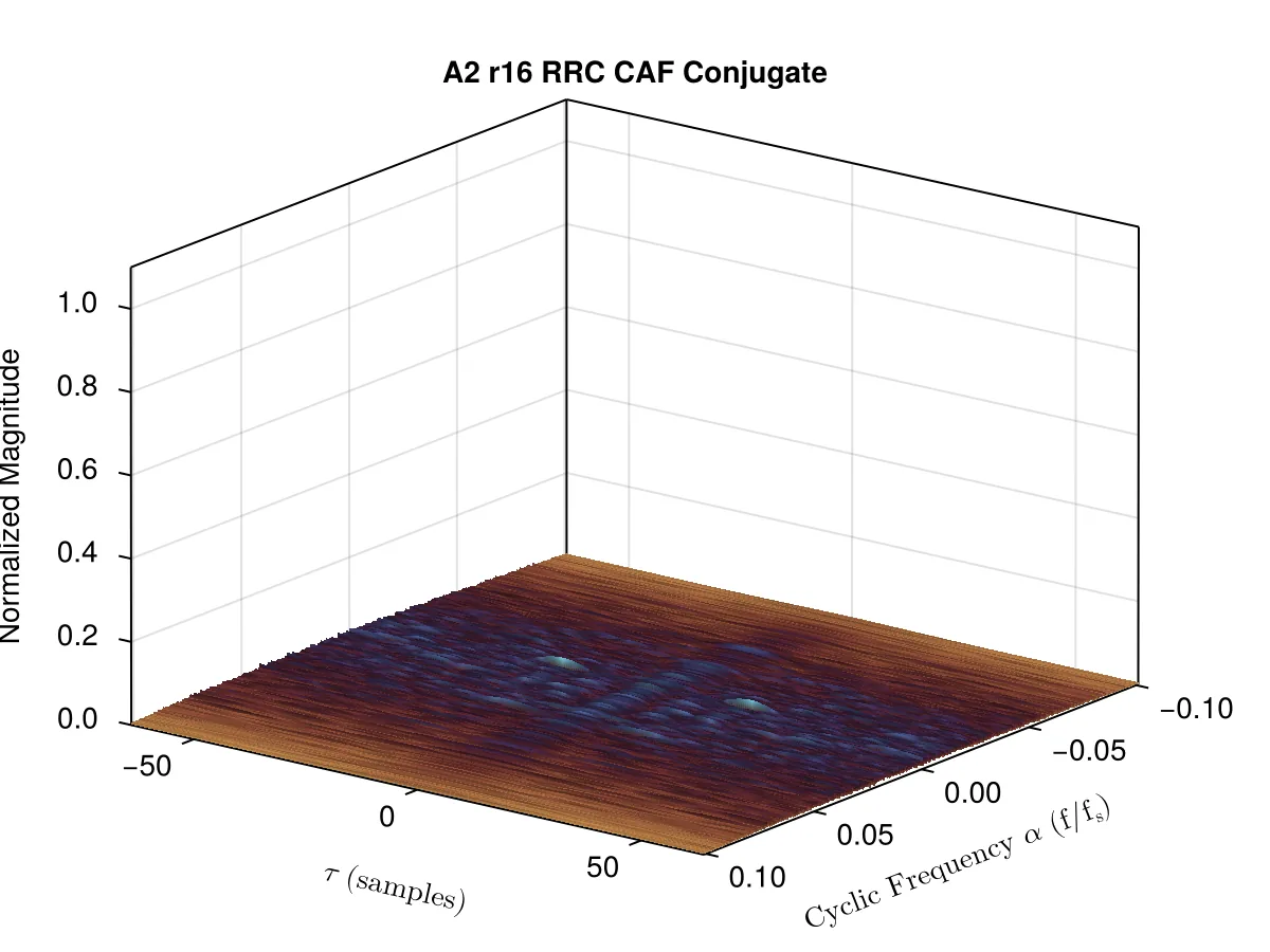
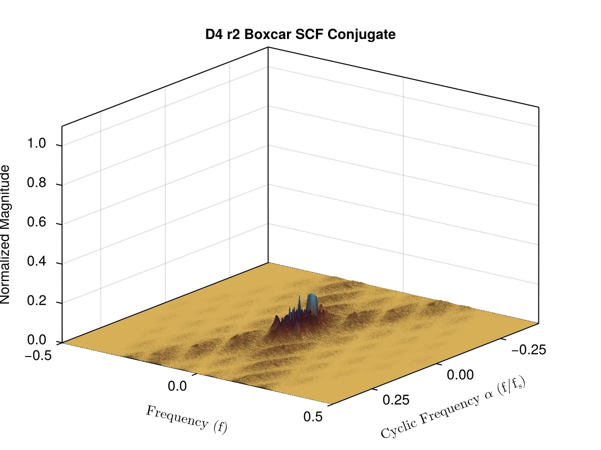
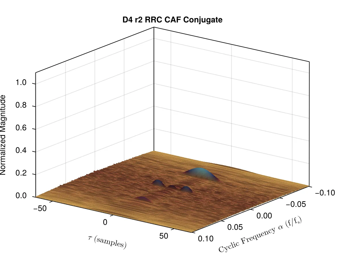
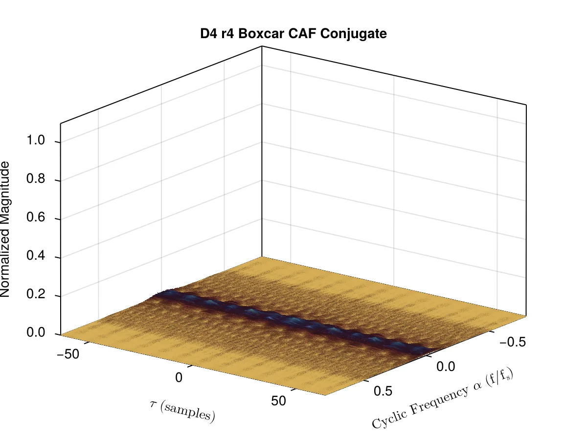
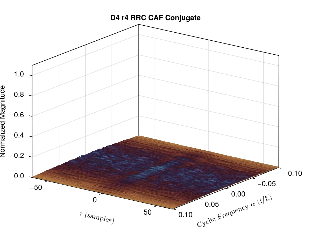
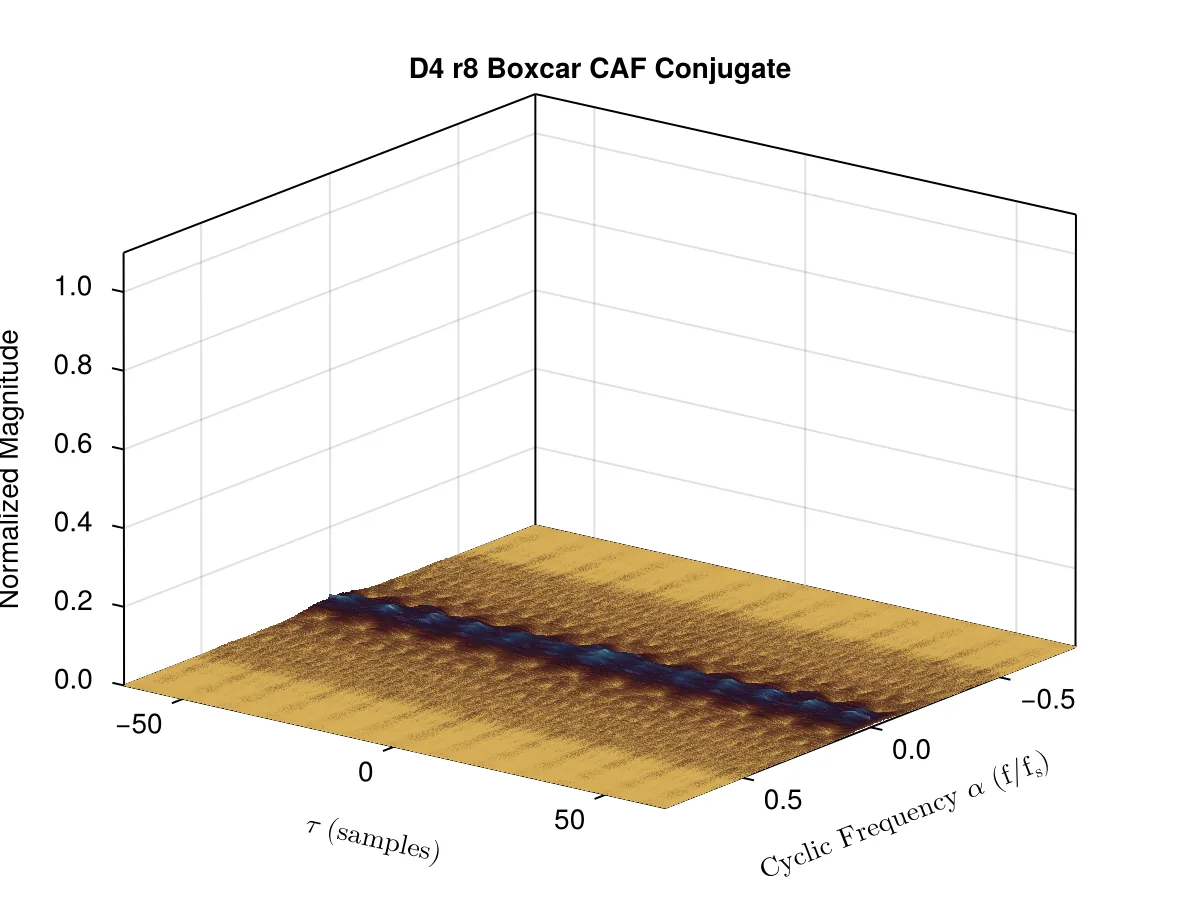
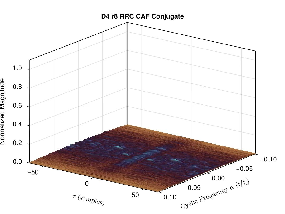
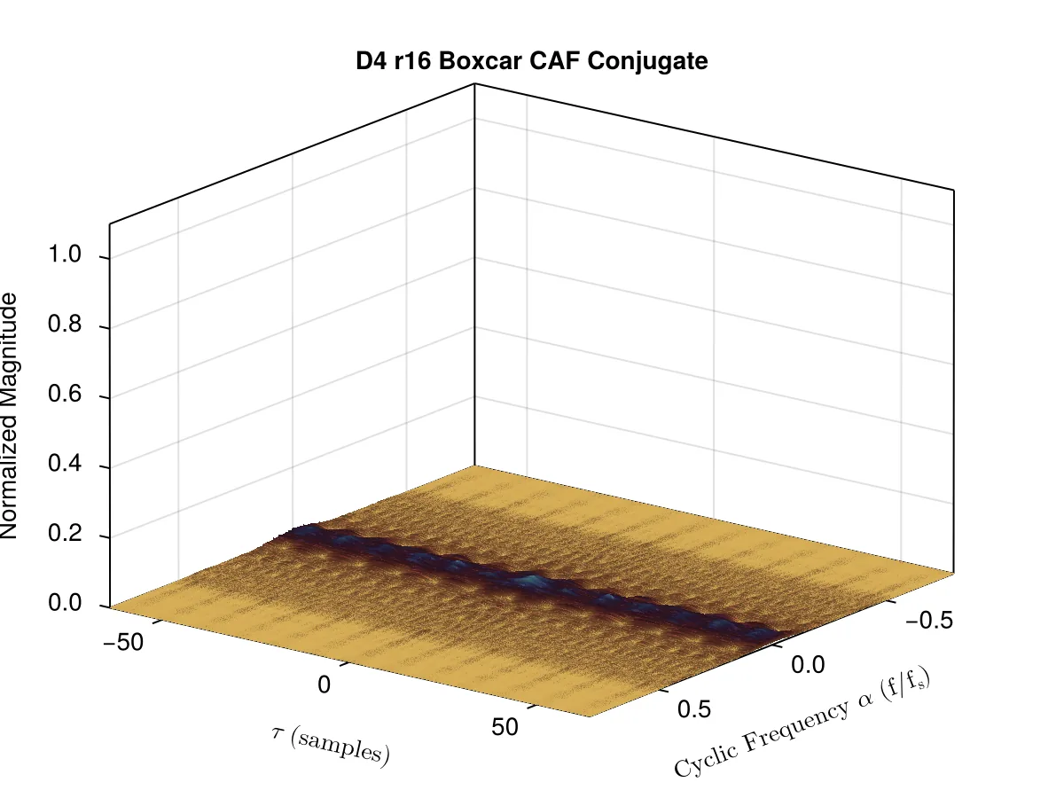
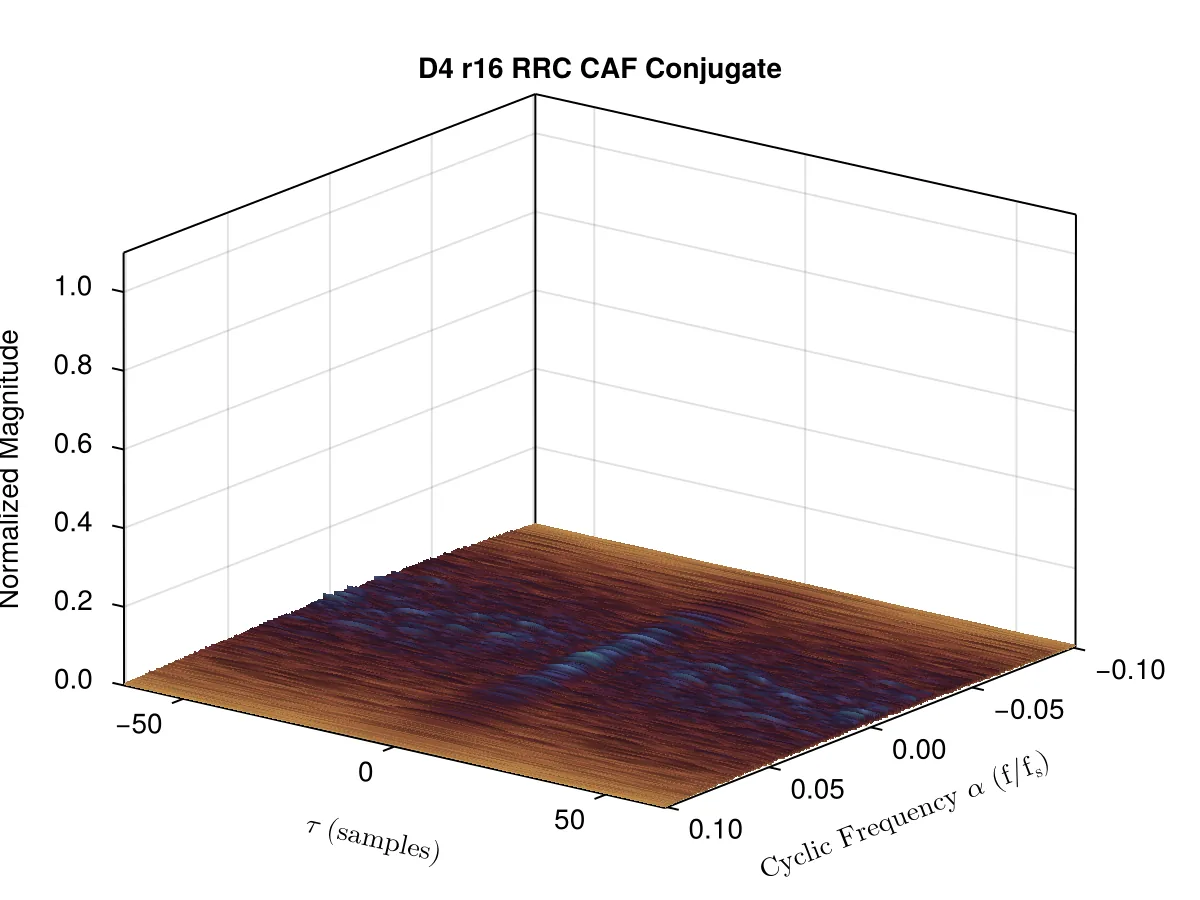
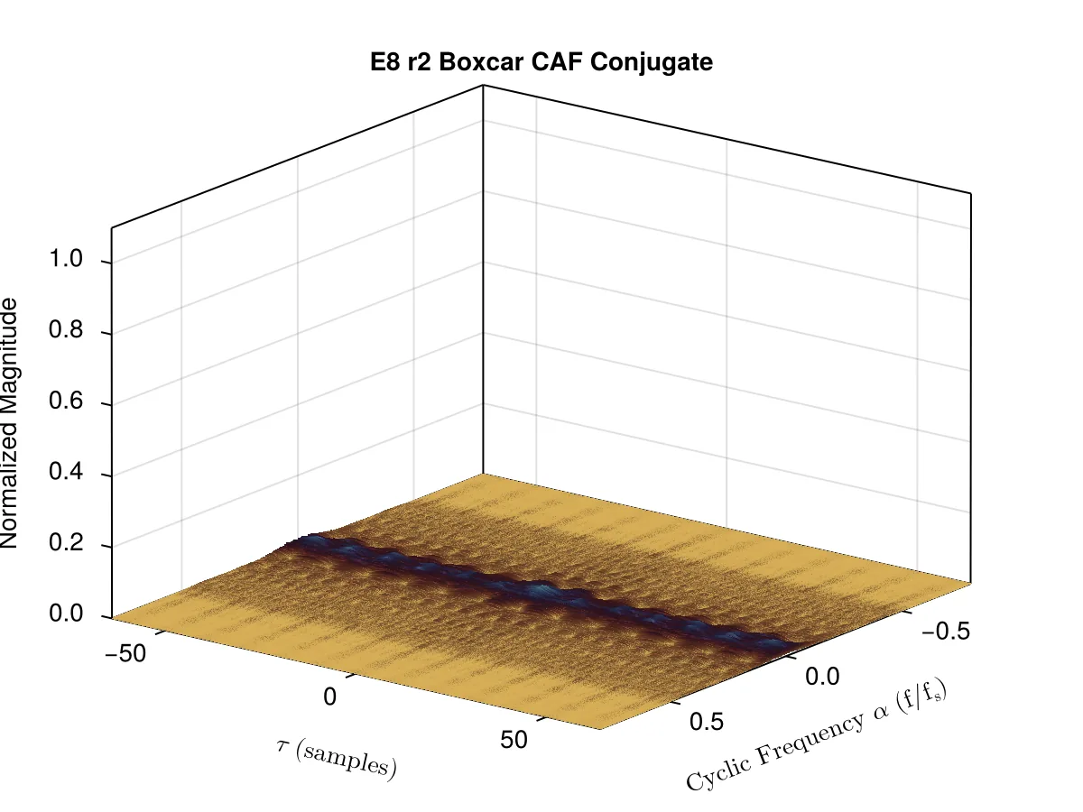
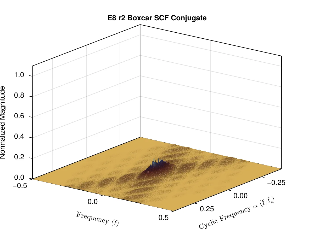
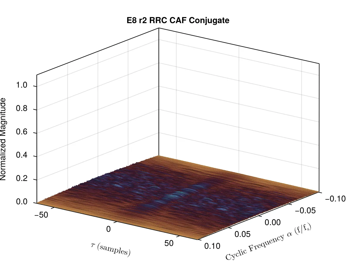
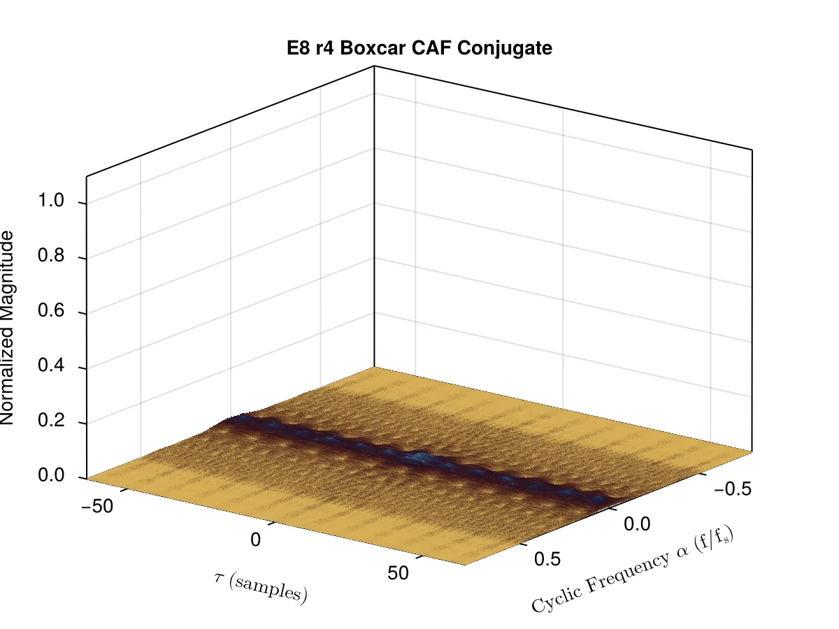
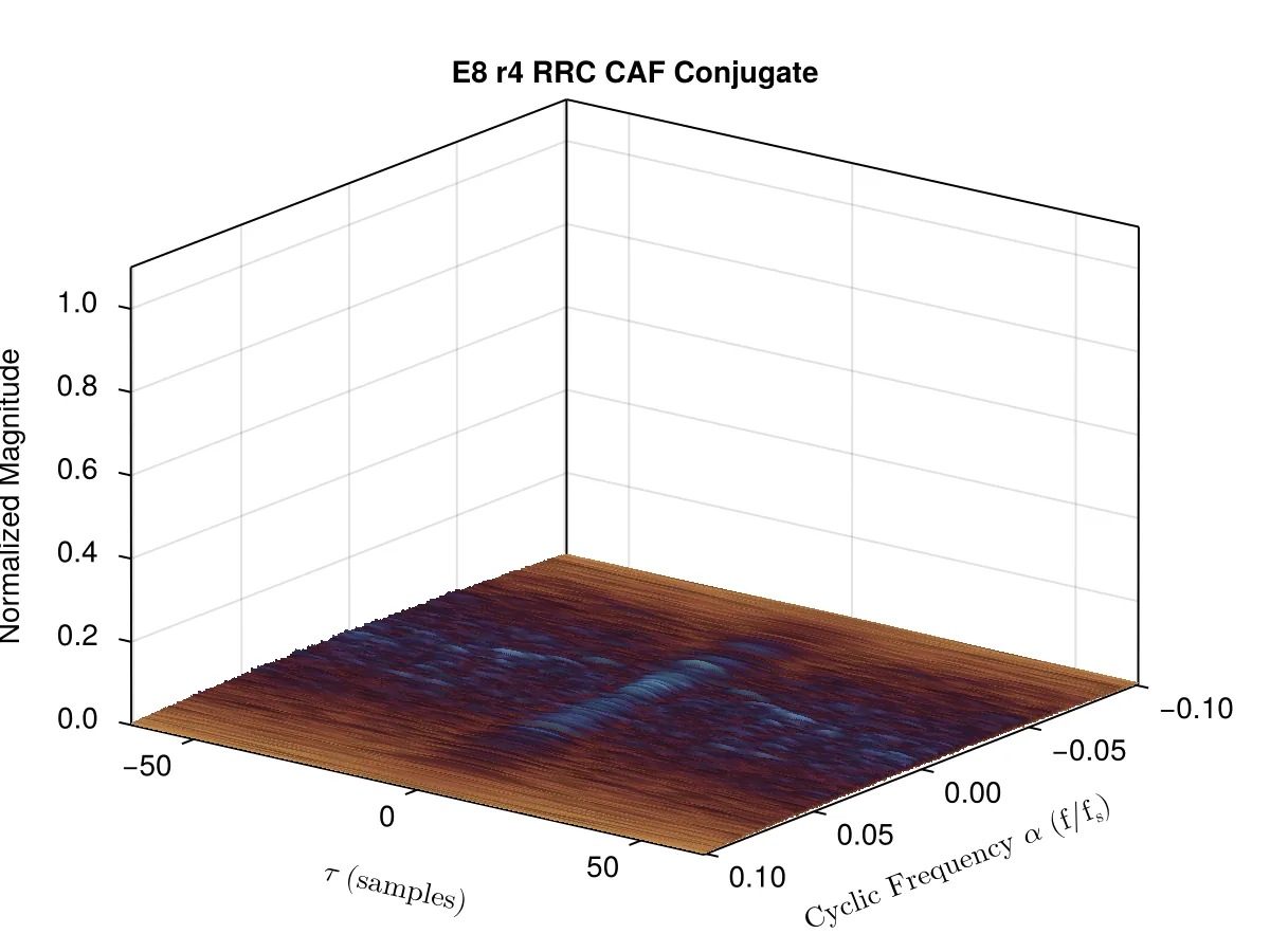
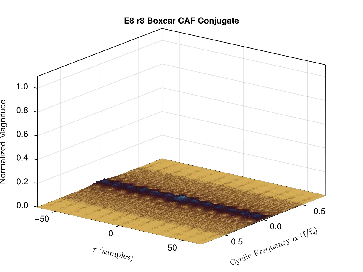
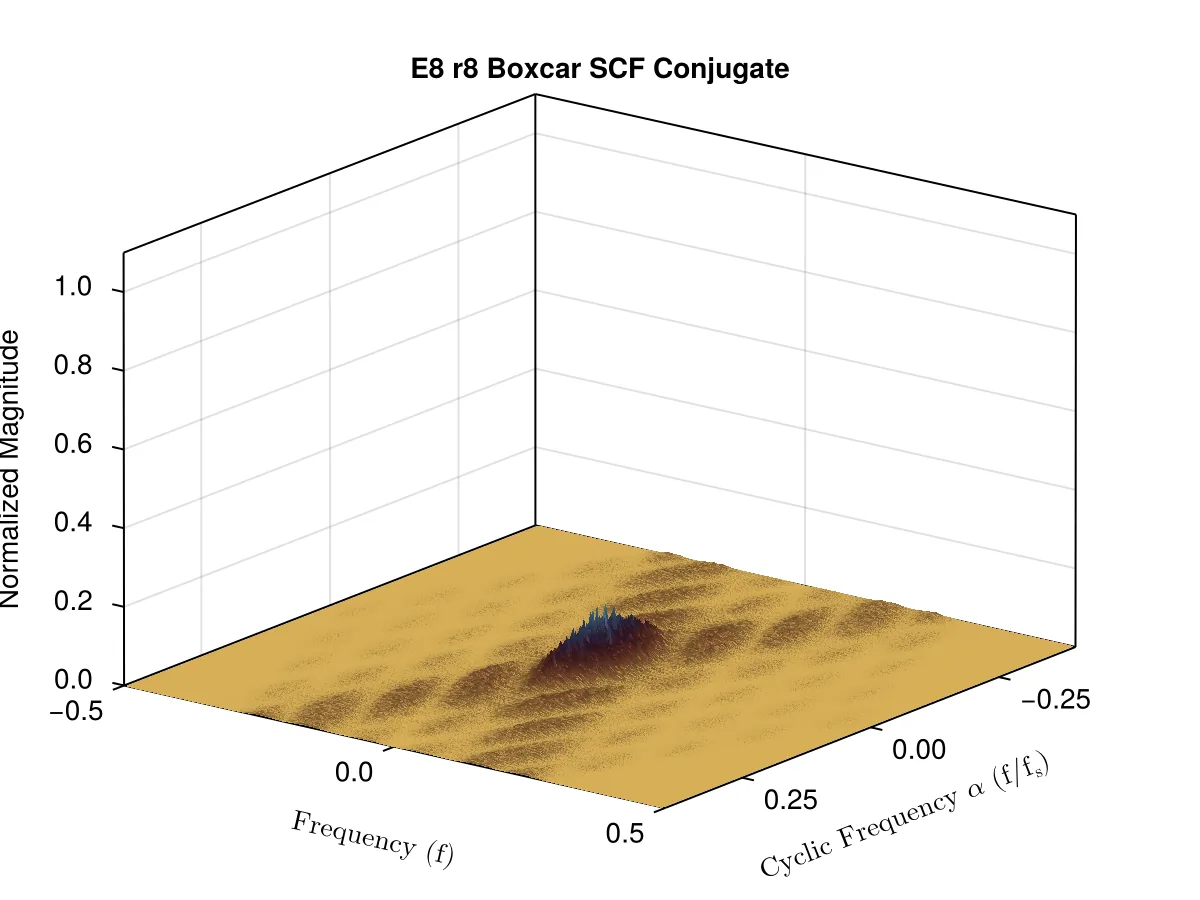
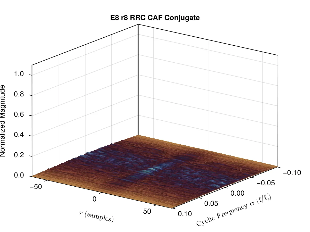
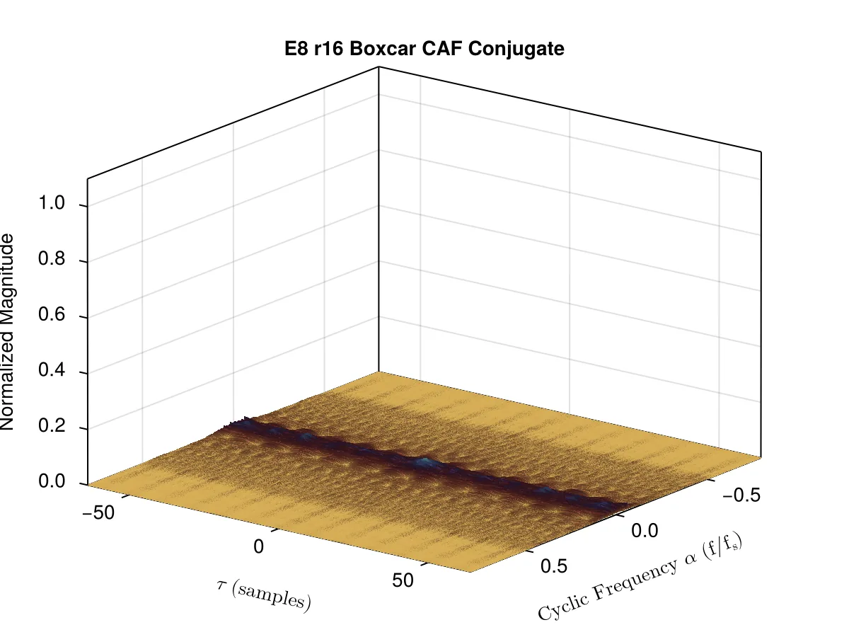
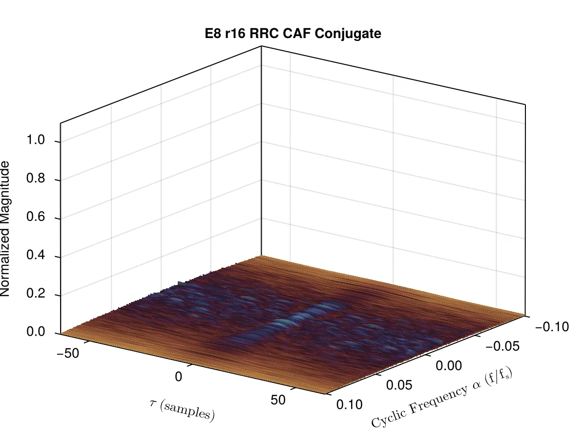
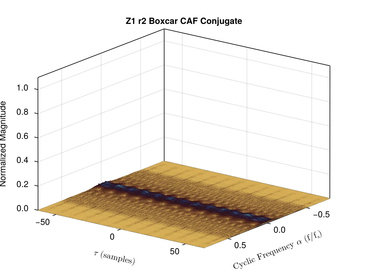
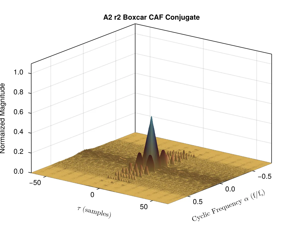
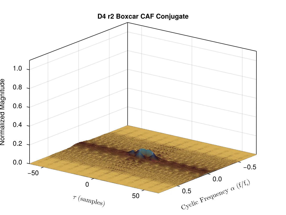
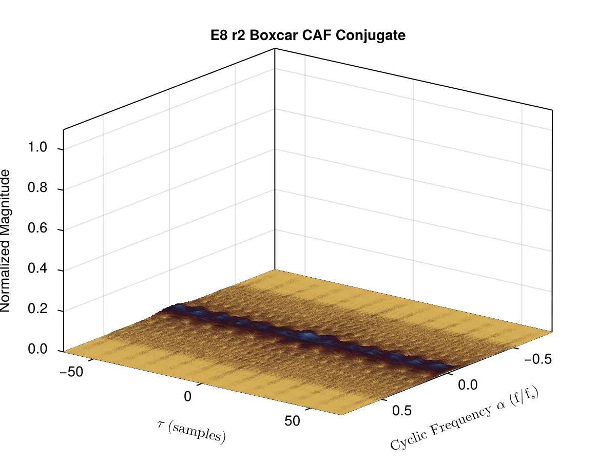
The CAF Conjugate highlights rotational asymmetry and is built using different variations of the second-order conjugate moment, E[s_n²]. When applied to the entire set of constellation IQ points, E[s_n²] provides a measure of structural imbalances across the real and imaginary axes. The magnitude of |E[s_n²]| should always lie between 0 and 1 when normalized by R_xx^(alpha=0)(tau = 0) and can give insight as to what we should expect to see in the CAF conjugate response. If |E[s_n²]| = 0, the signal shows perfect rotational symmetry and the CAF Conjugate will look indistinguishable from the noise floor. At 1, the signal has maximum asymmetry and the CAF Conjugate has more distinguishable peaks and hills. Between 0 and 1, the constellation is two-dimensional but warped, stretched, or unevenly distributed. The one exception to this is if you need to rotate 180 degrees to line up constellation points, such as a BPSK signal. For this case of rotational symmetry only, constellation points collapse to a single phase and will sum coherently, maximizing the second-order conjugate moment.
BPSK and QPSK are often used to show these extremes.

BPSK:  E[s_n²] = (½) [ (-1)² + 1² ] = 1
QPSK:  E[s_n²] =(¼) [(-0.5-0.5i)² + (0.5-0.5i)² + (-0.5+0.5i)² + (0.5+0.5i)²] = 0

Due to BPSK’s unique interaction with the second order conjugate moment, its CAF Conjugate plots for boxcar and RRC pulse shaping filters demonstrate peaks just as prevalent as its regular CAF response. QPSK, however, appears to look like Gaussian noise, regardless of filter type.

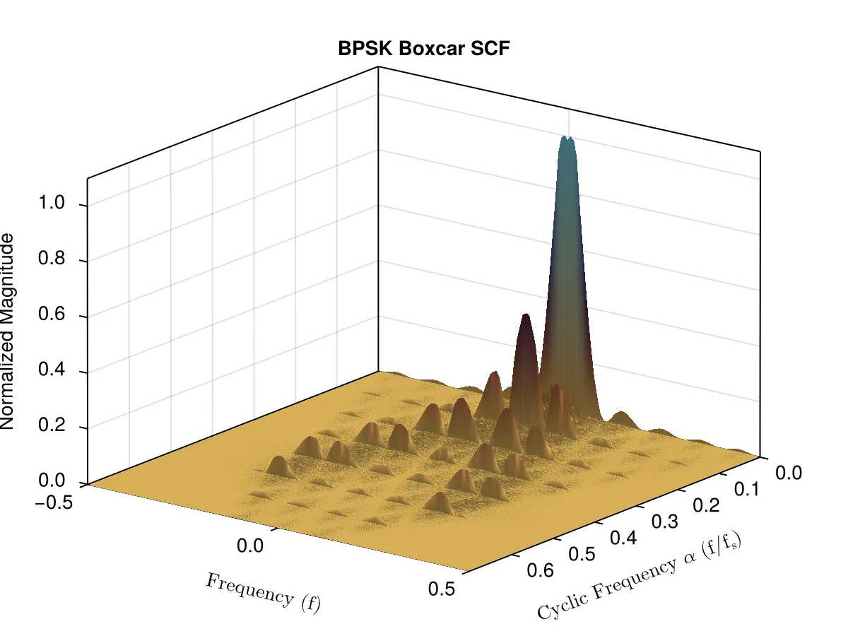
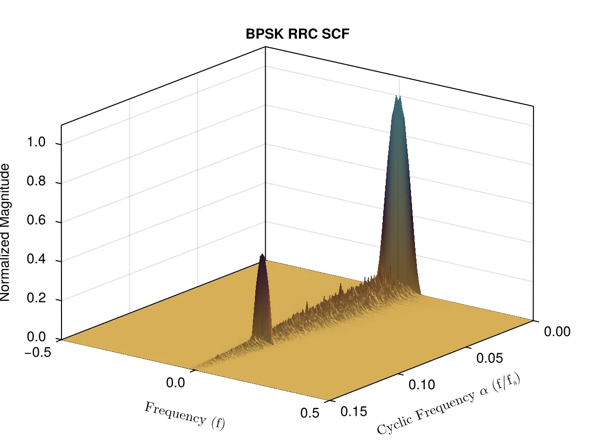
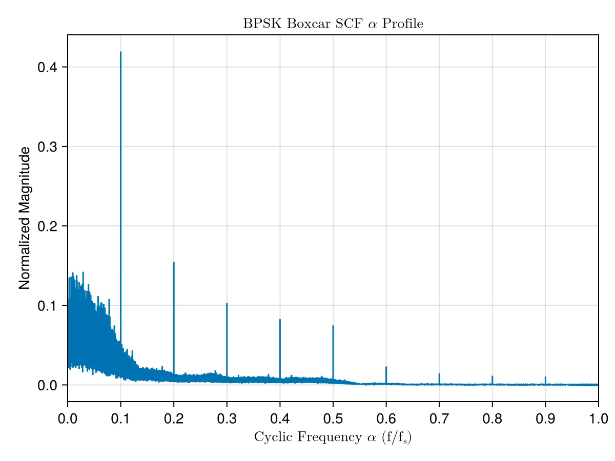
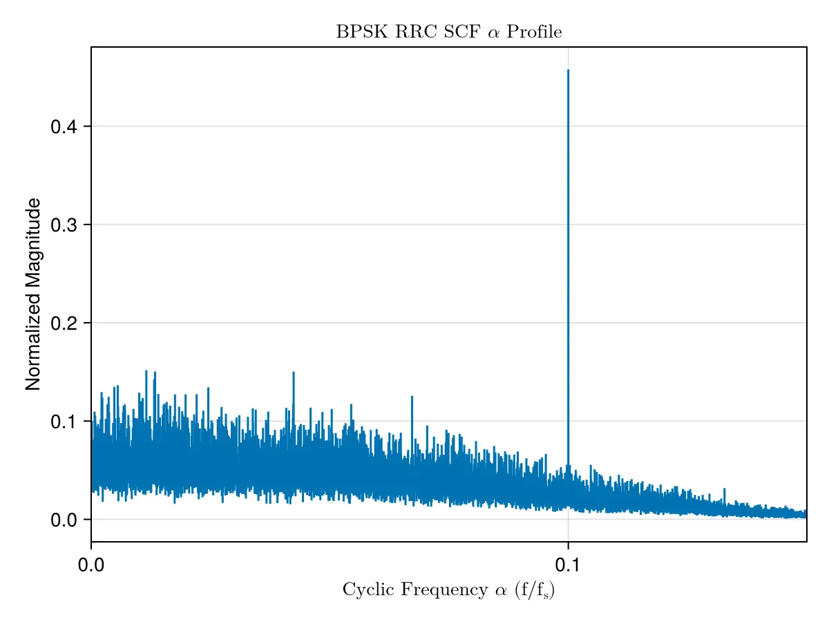
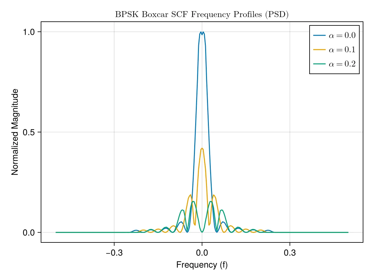
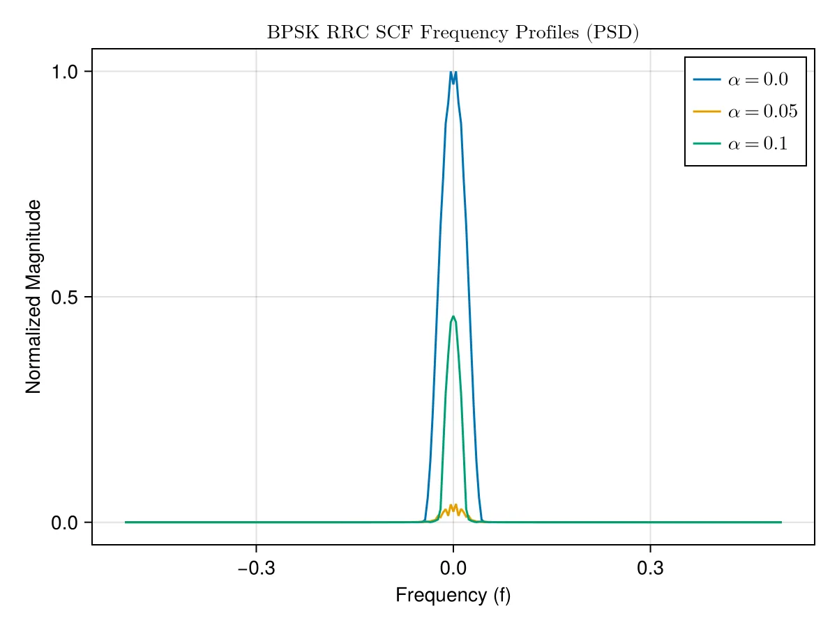
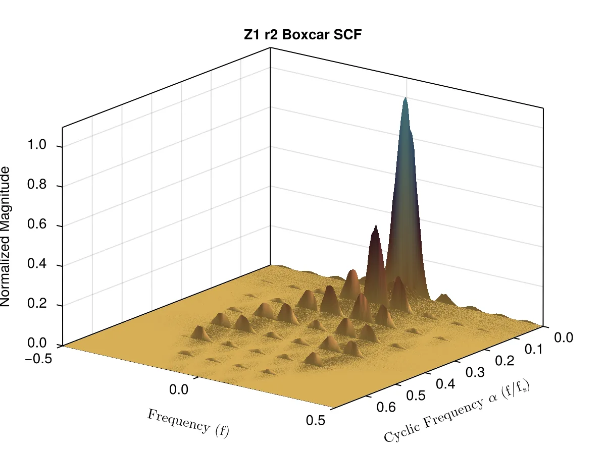
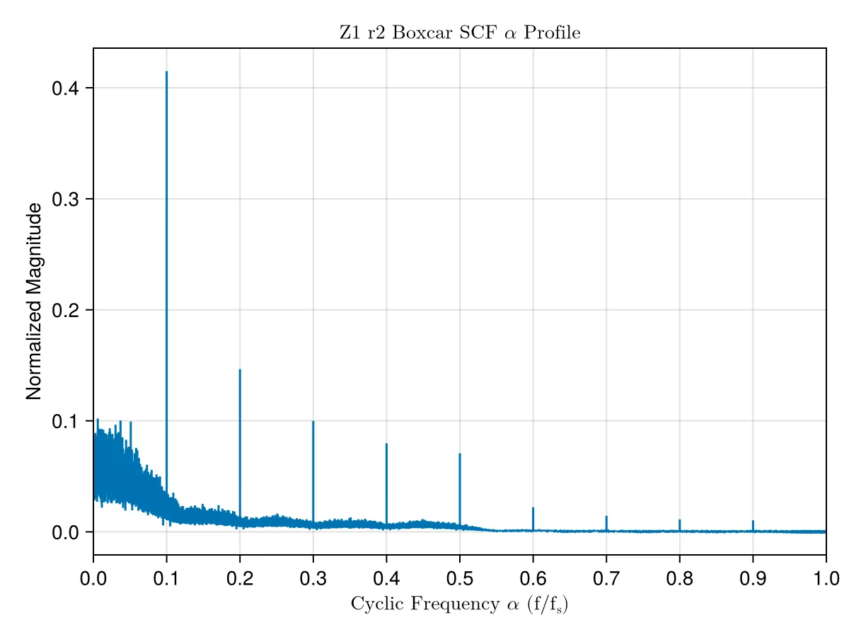
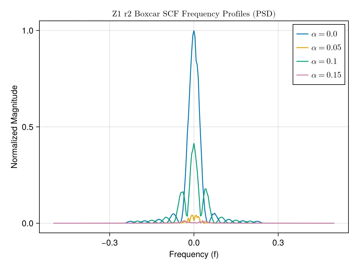
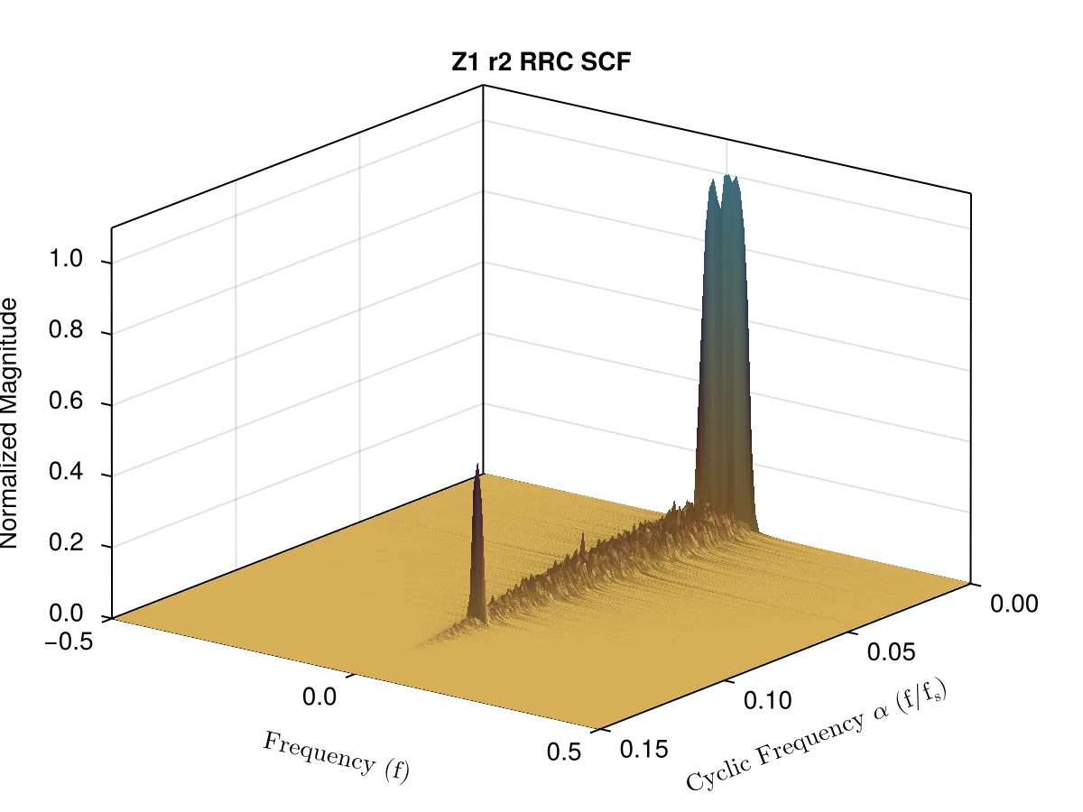
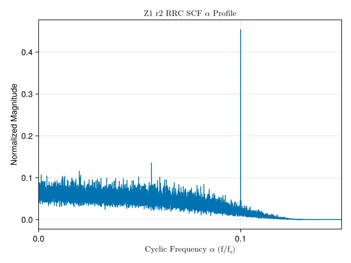
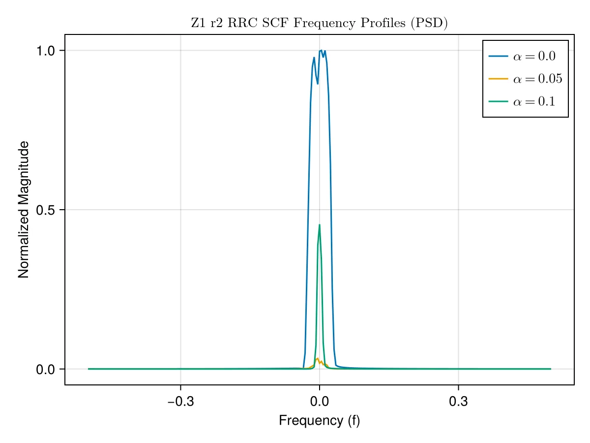
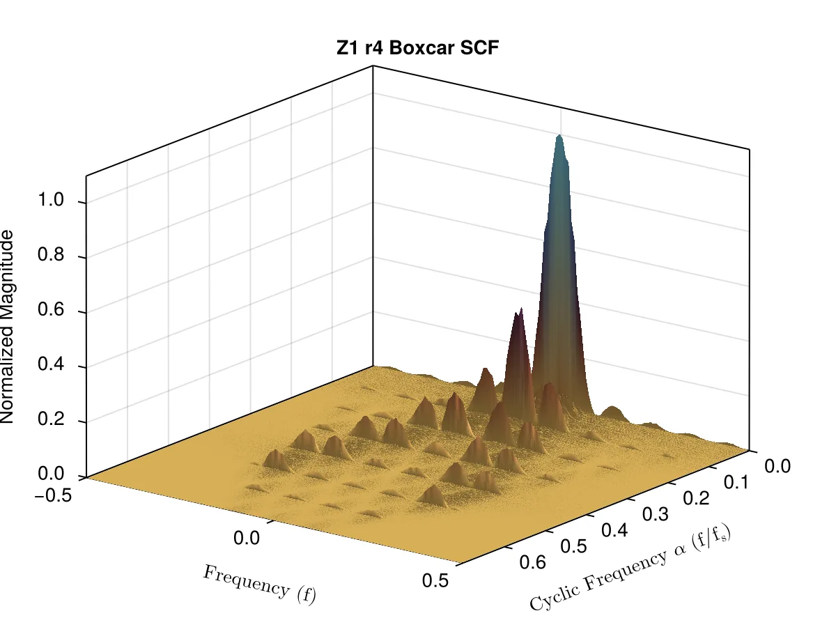
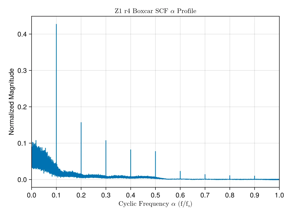
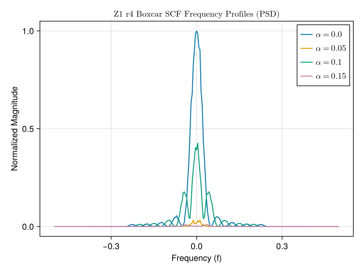
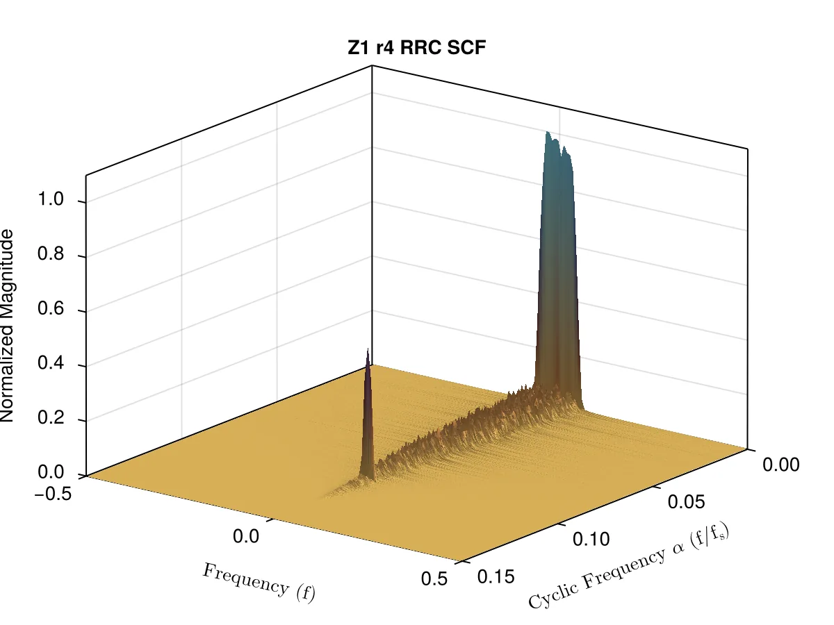
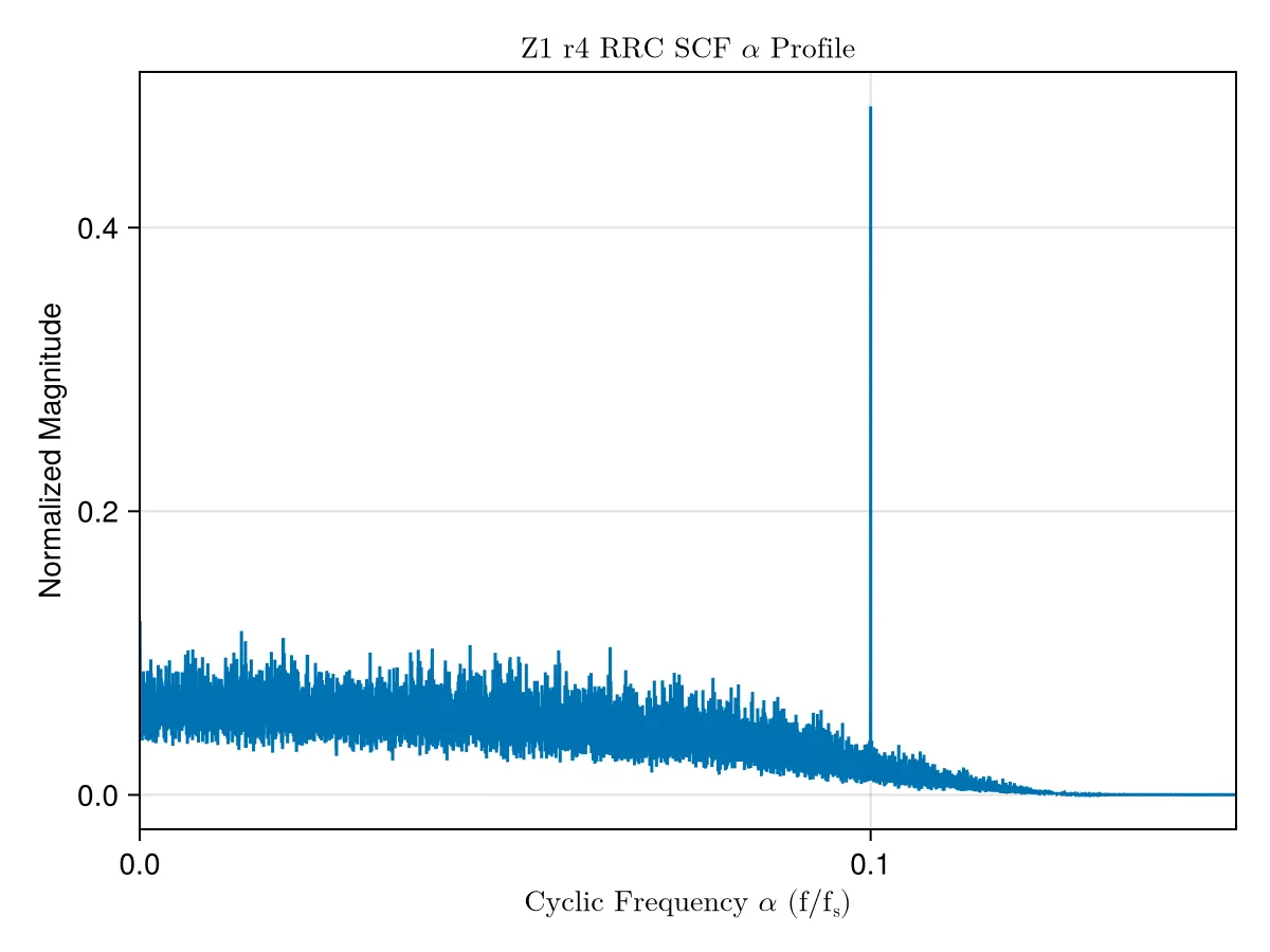
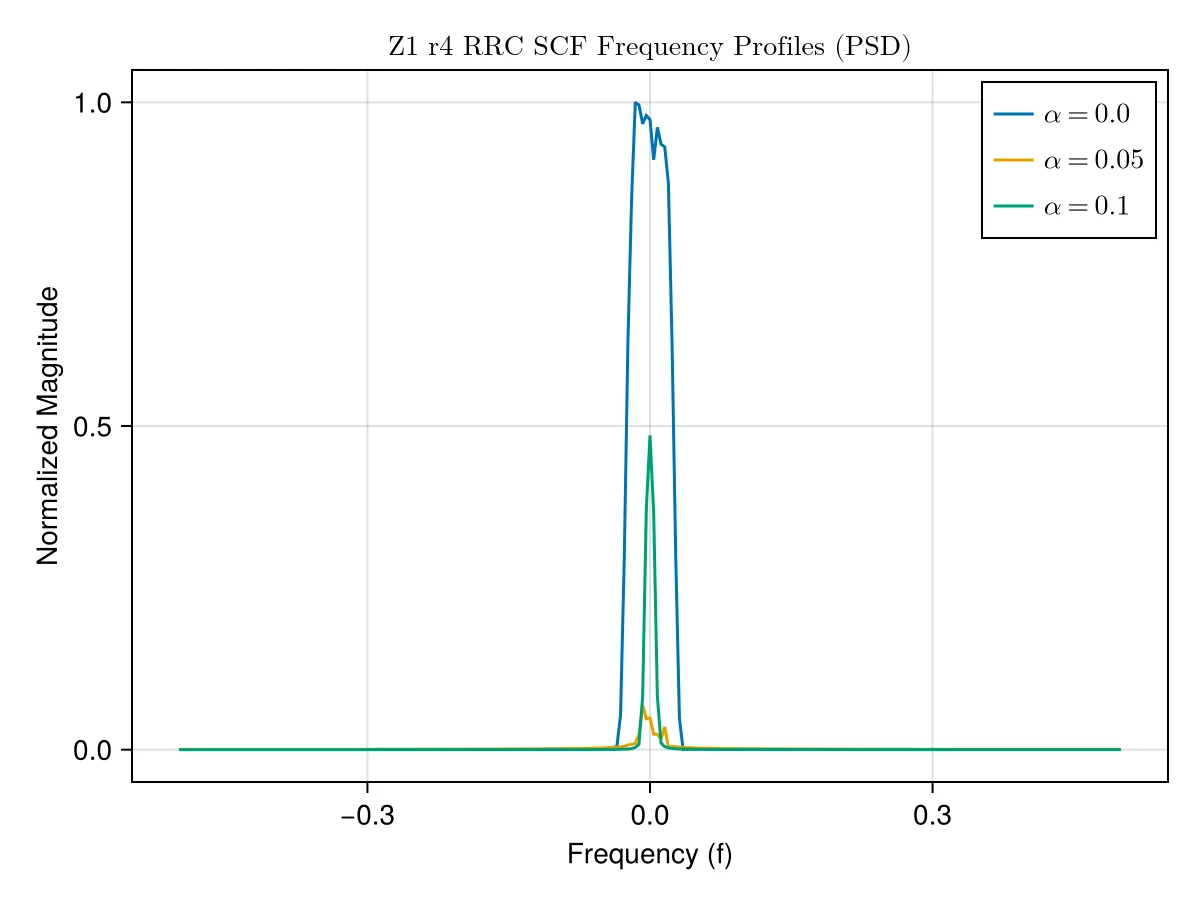
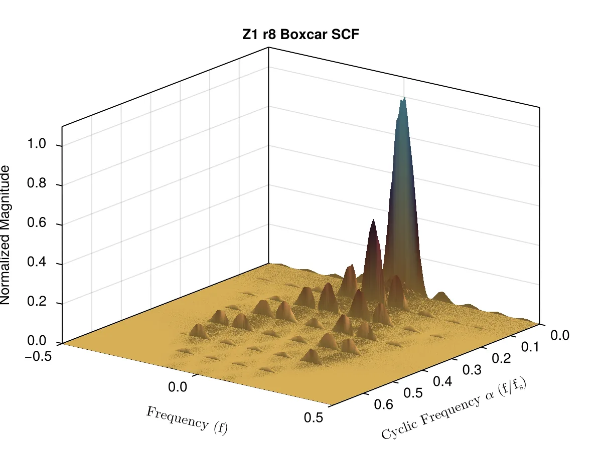
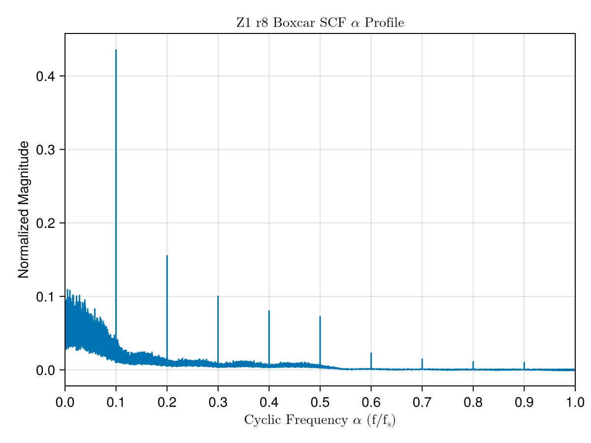
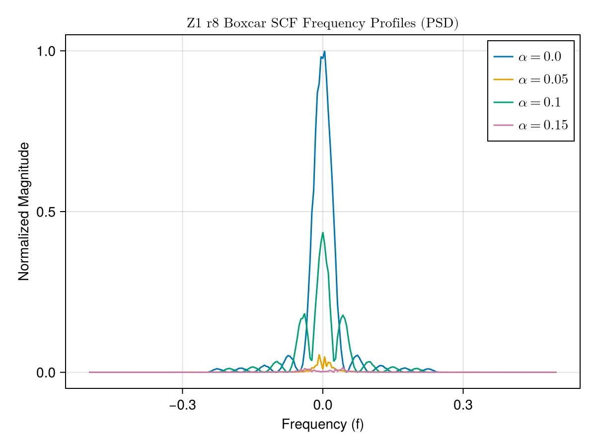
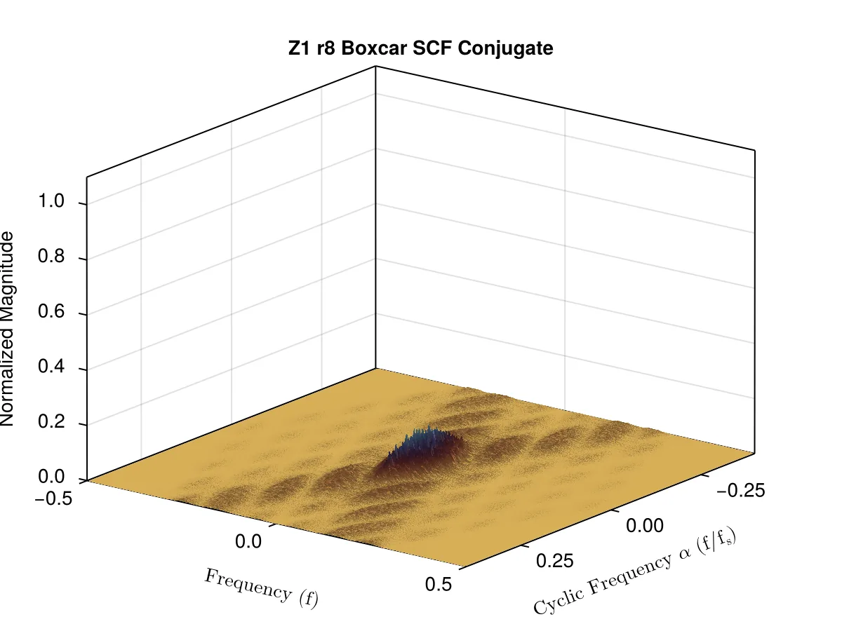
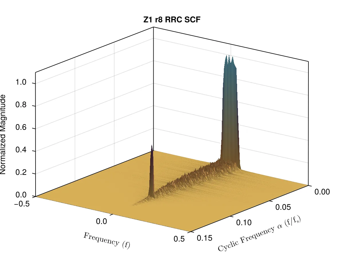
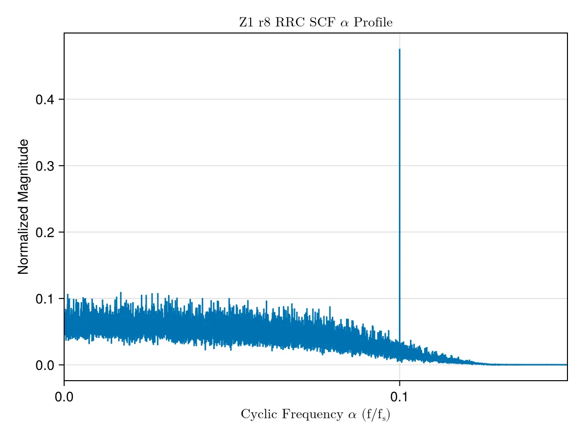
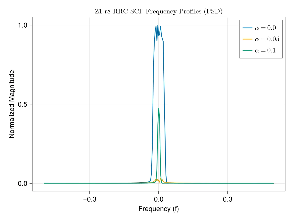
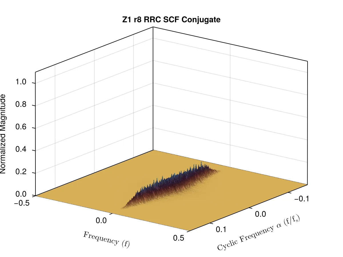
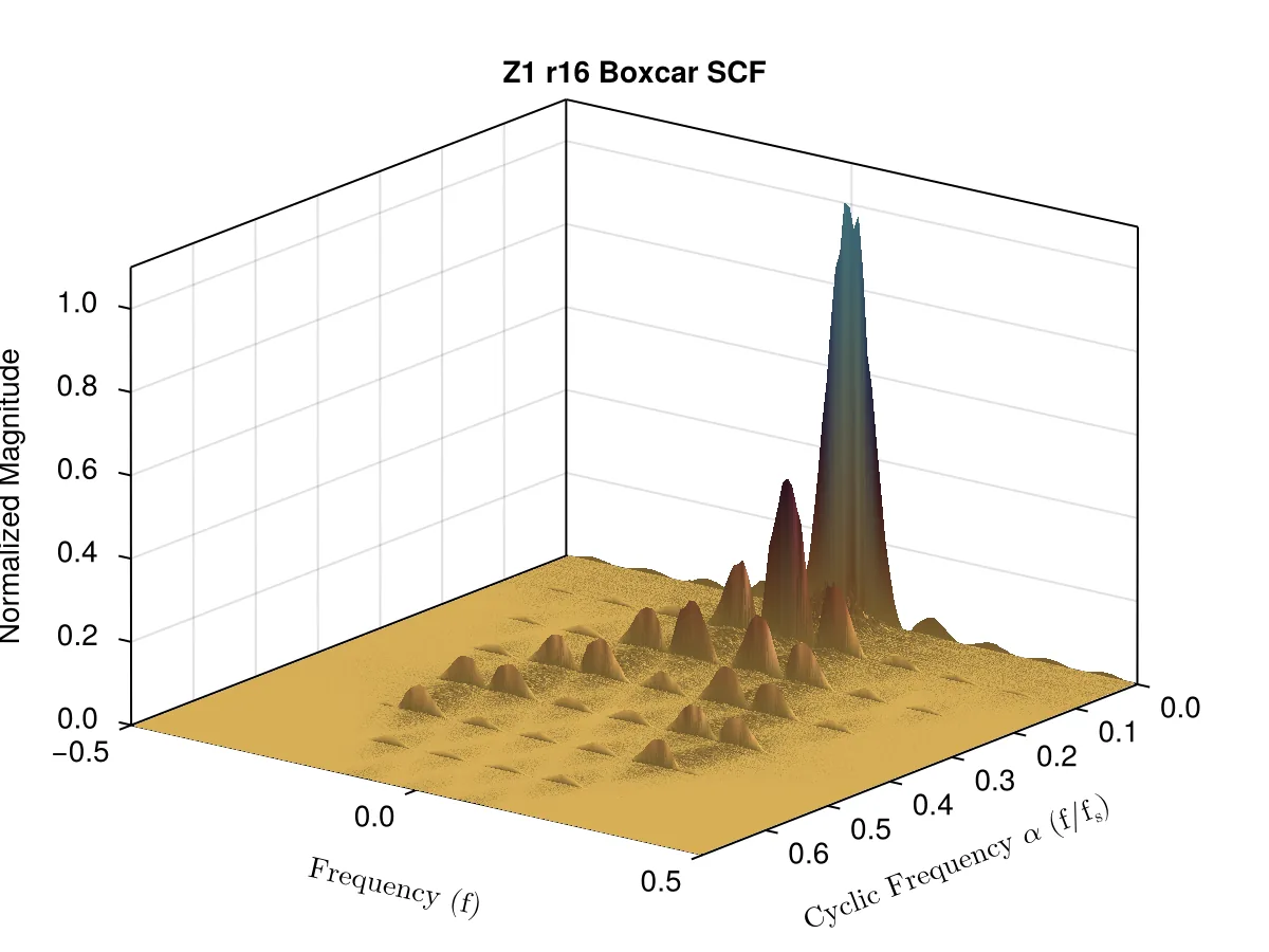
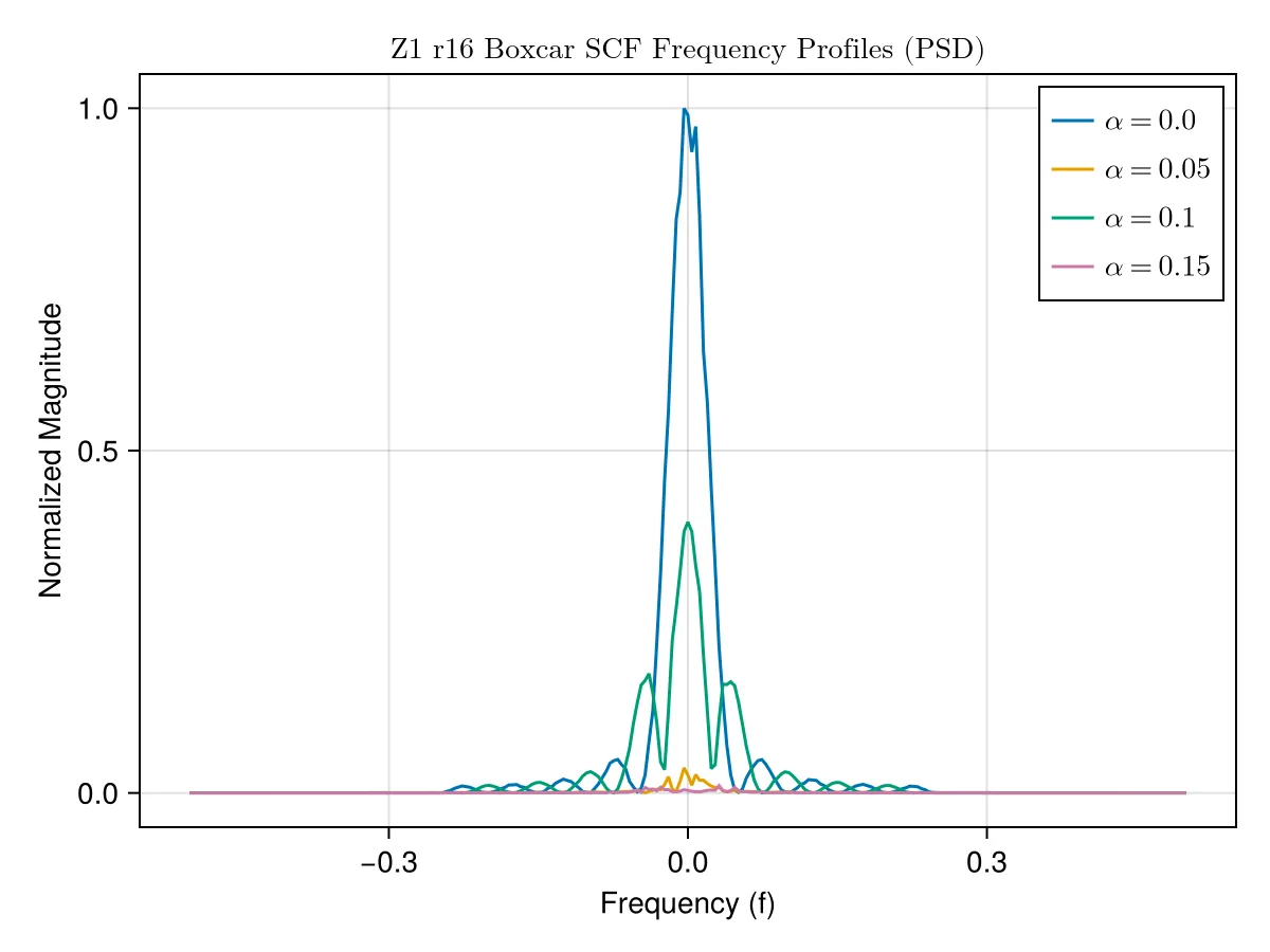
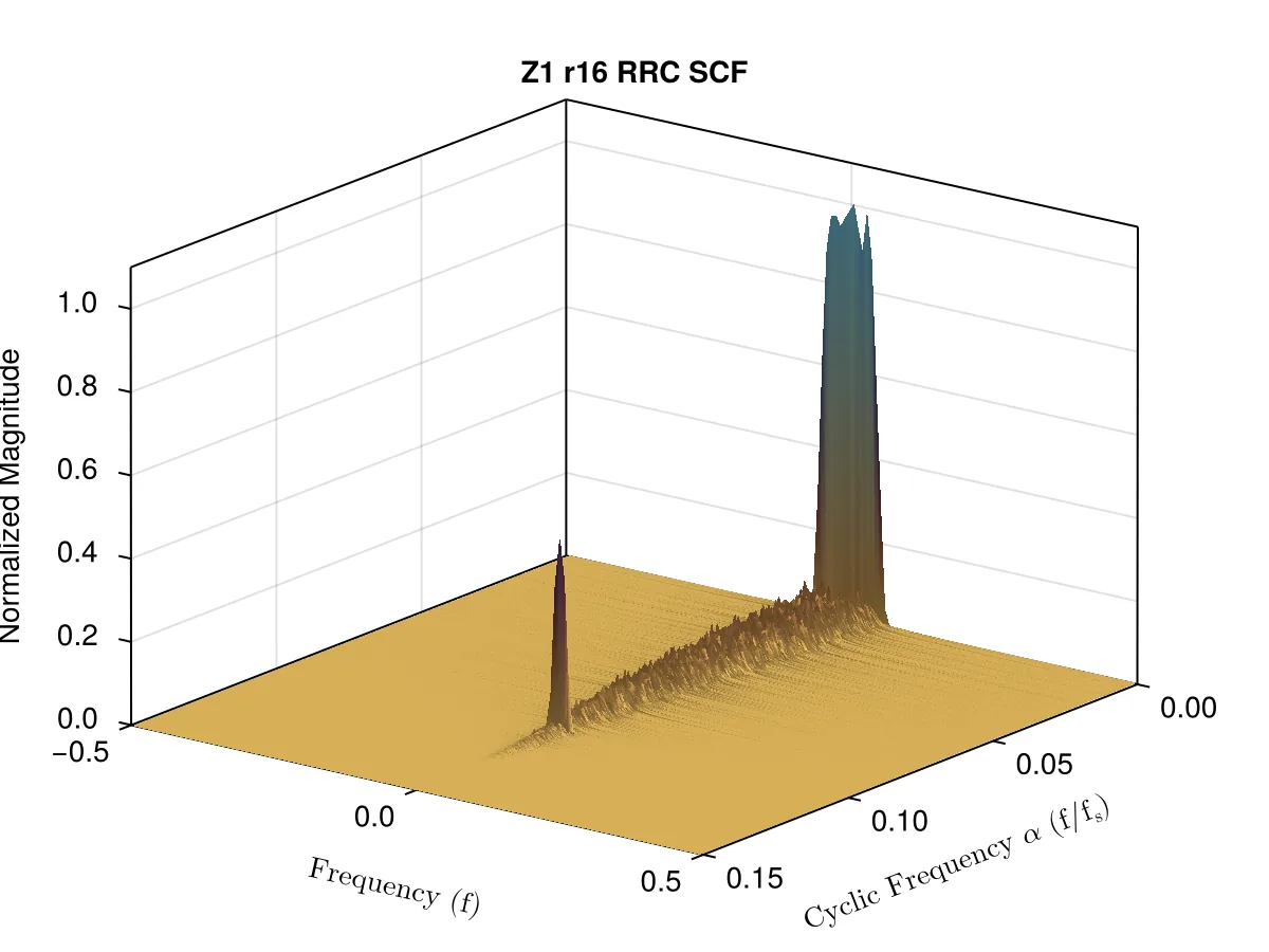
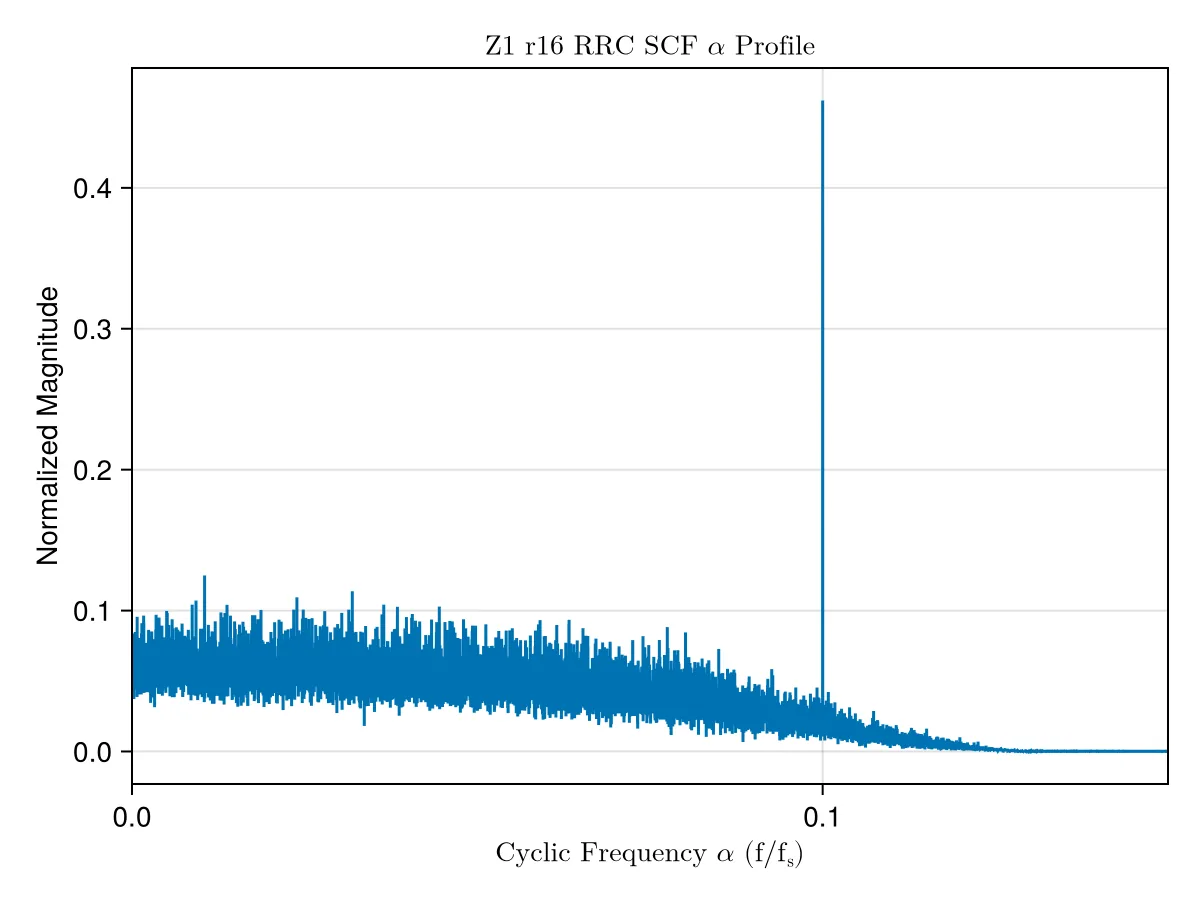
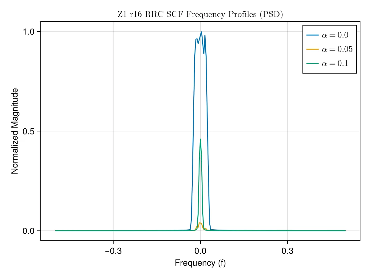
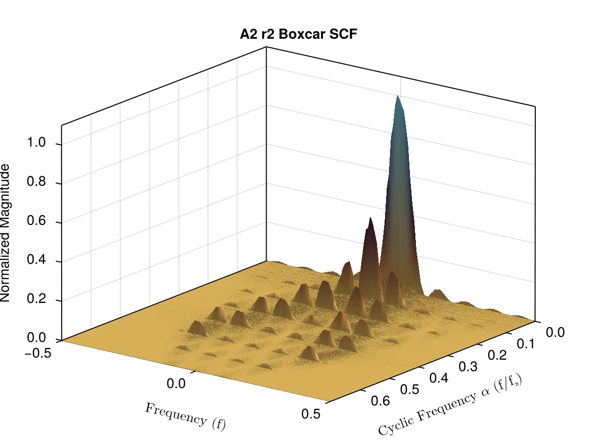
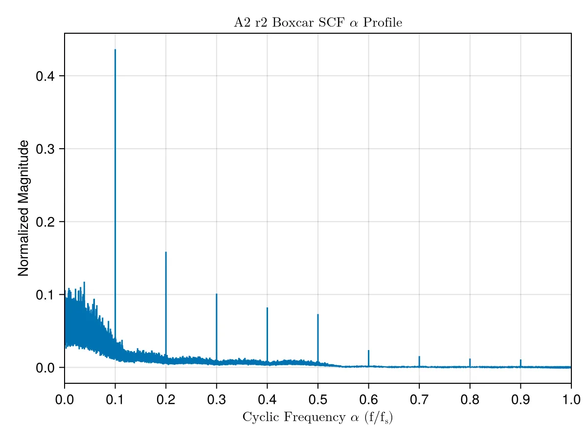
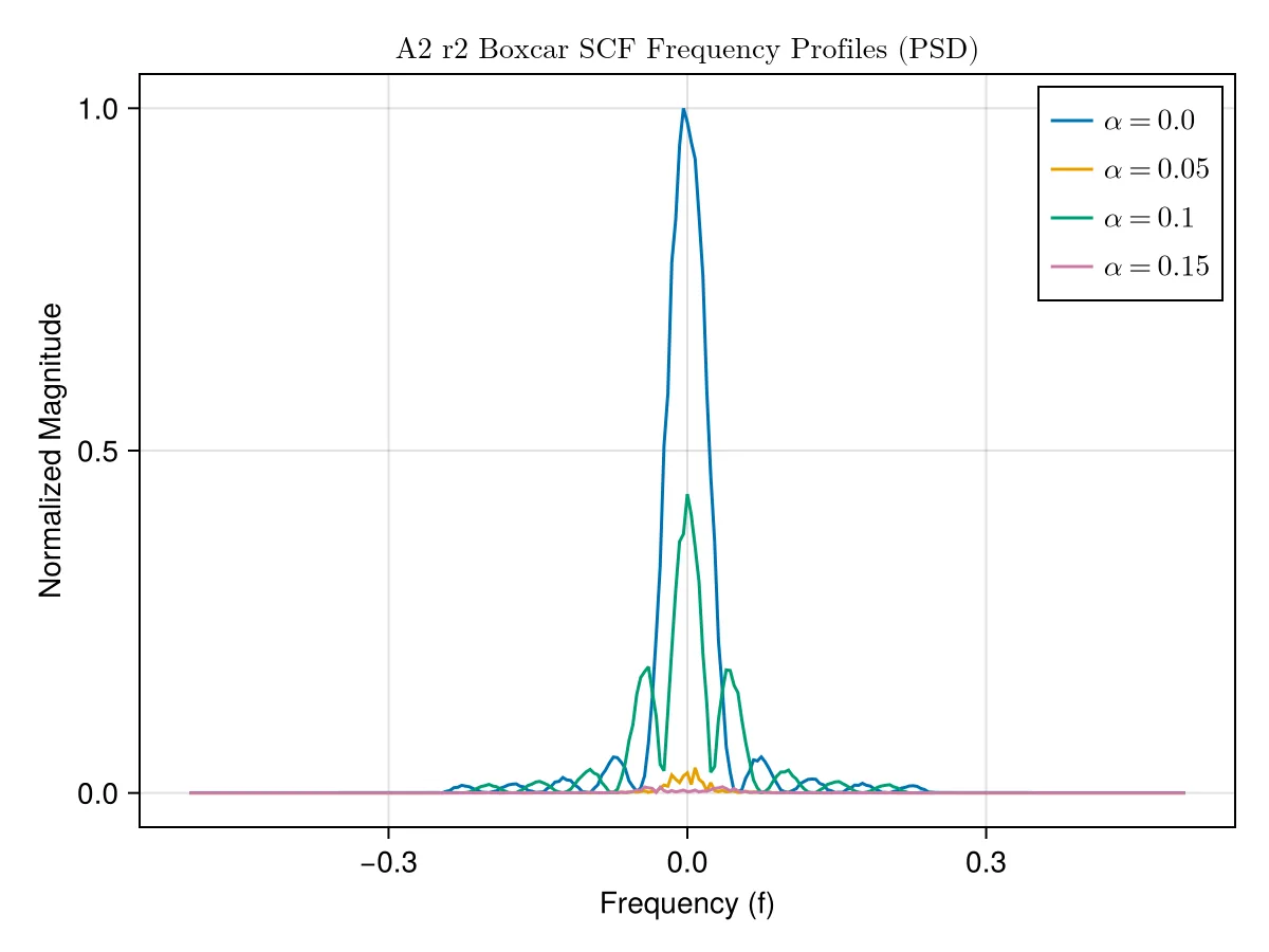
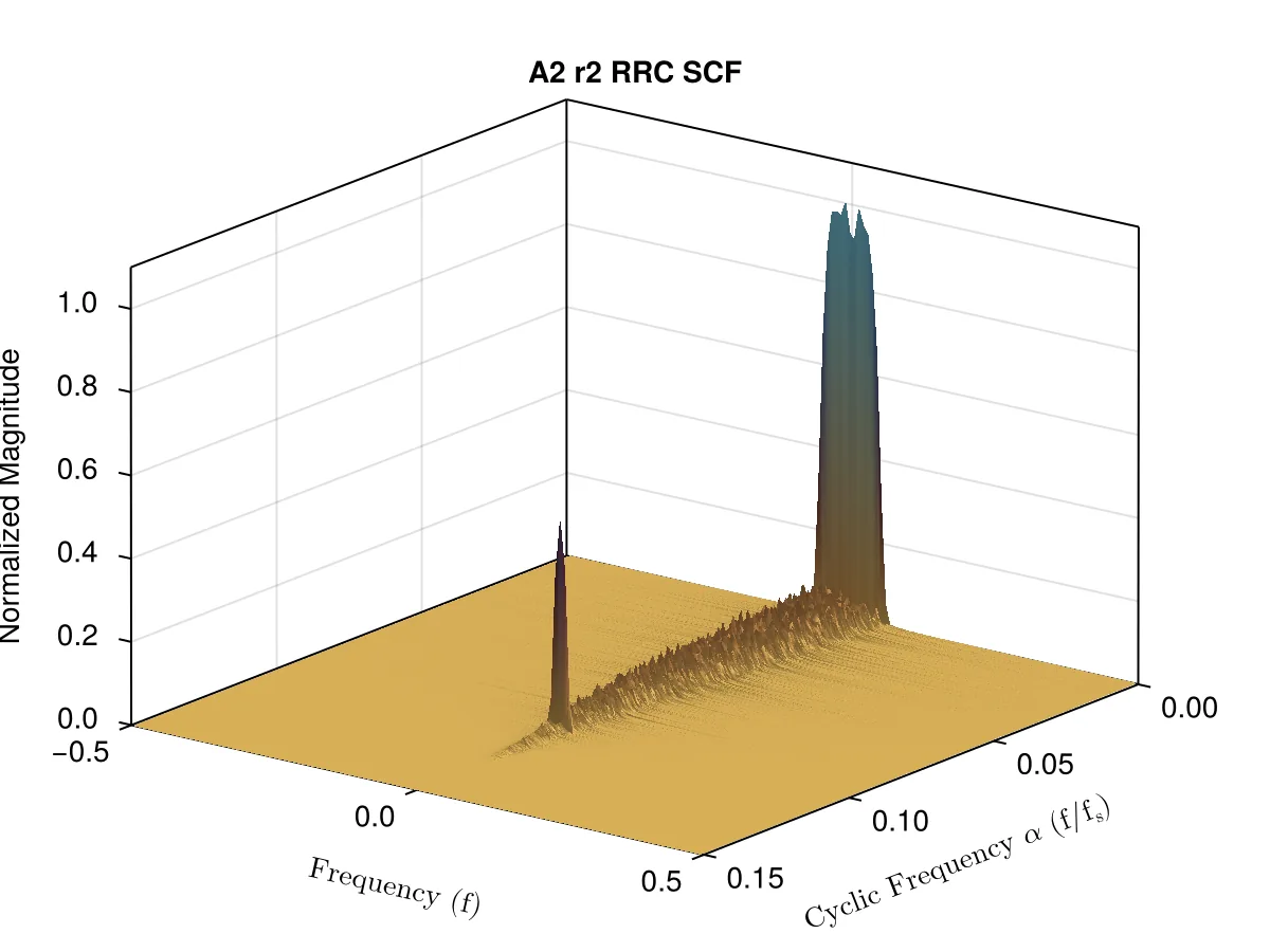
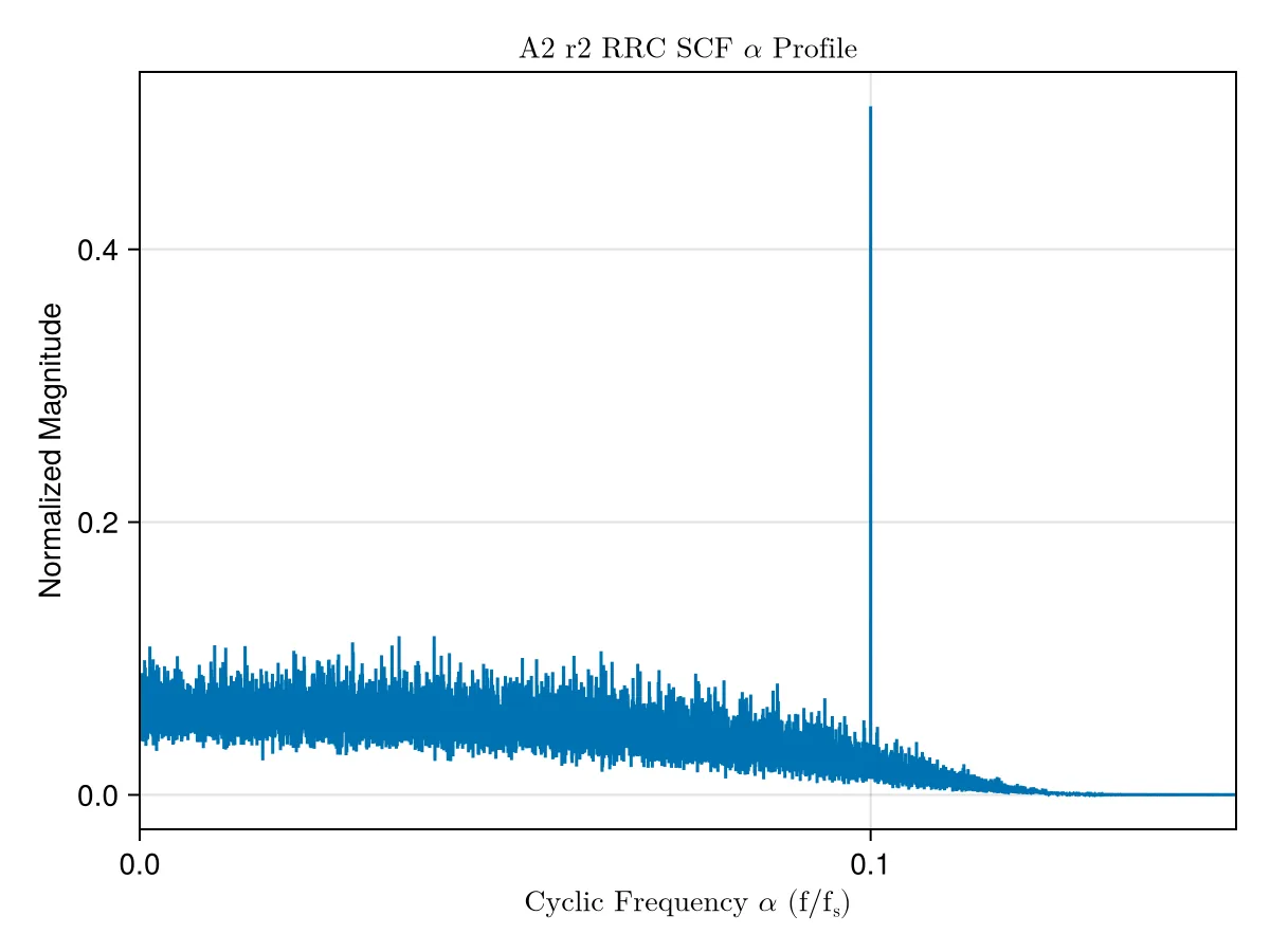
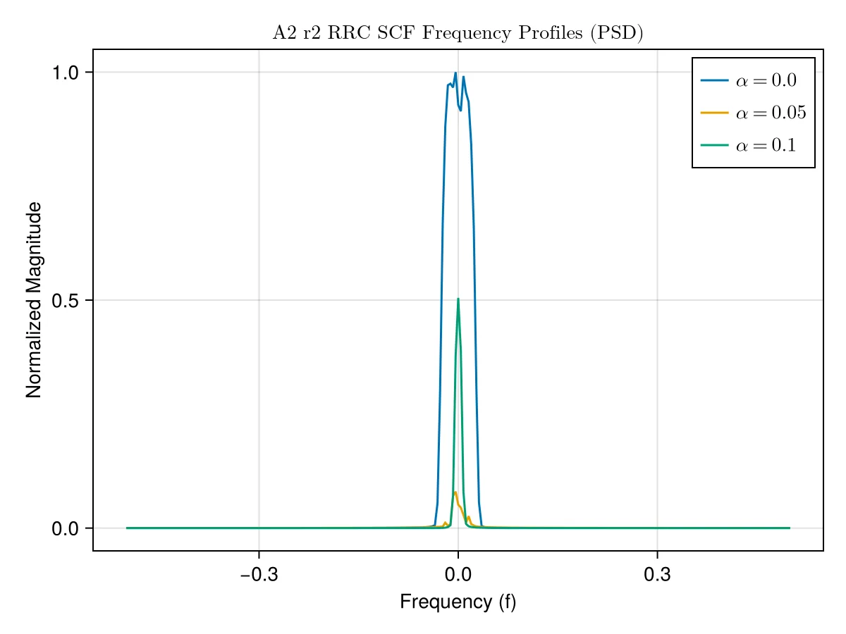
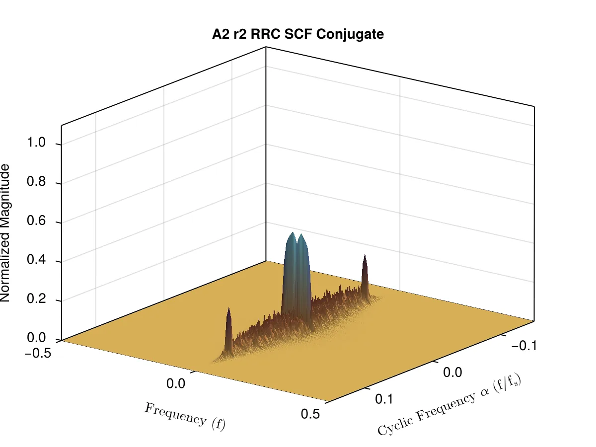
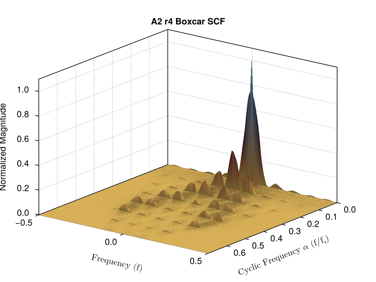
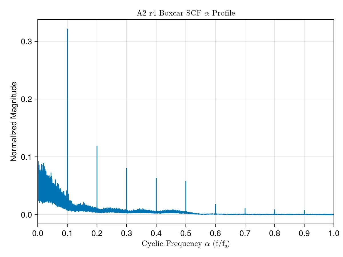
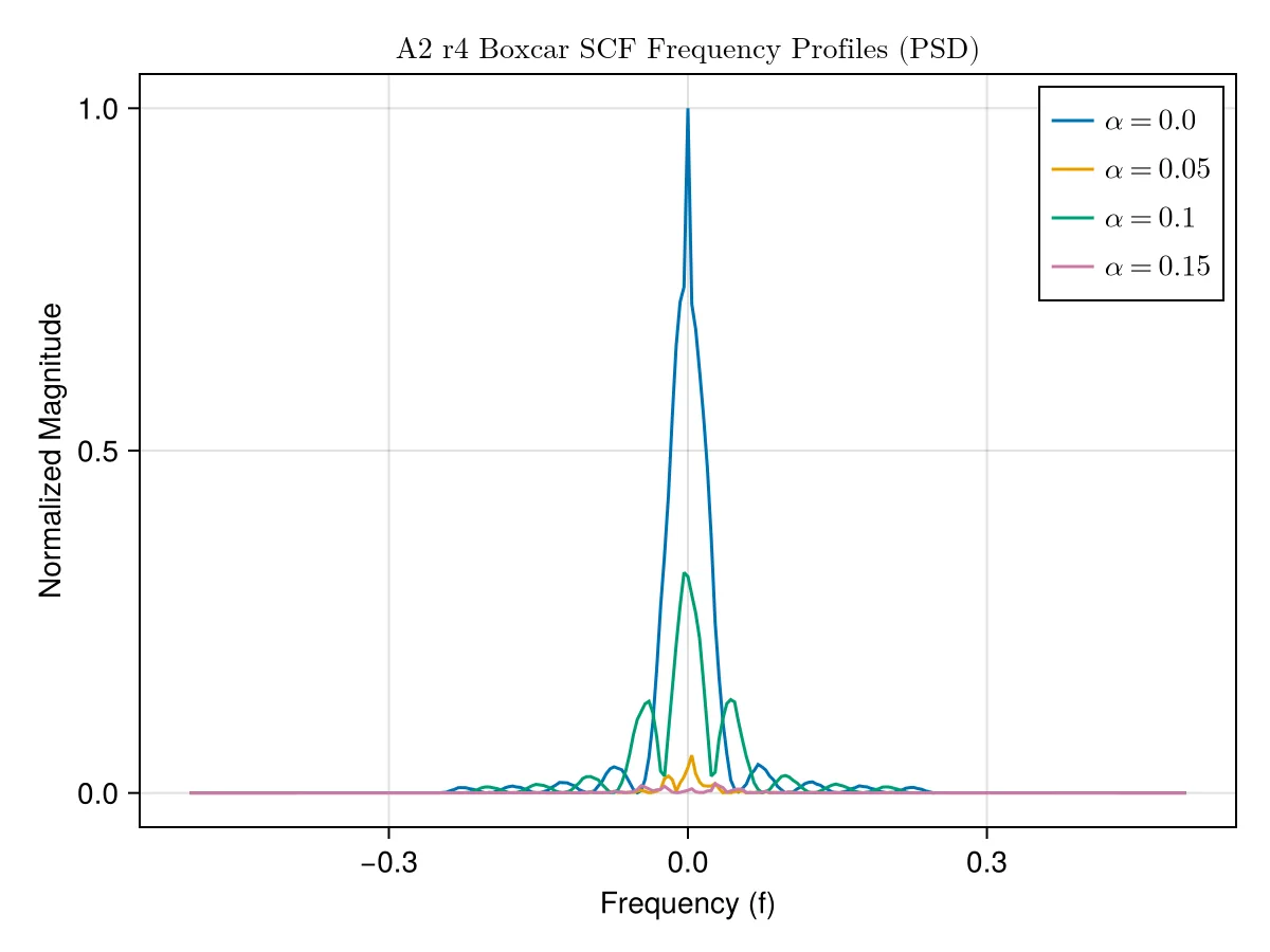
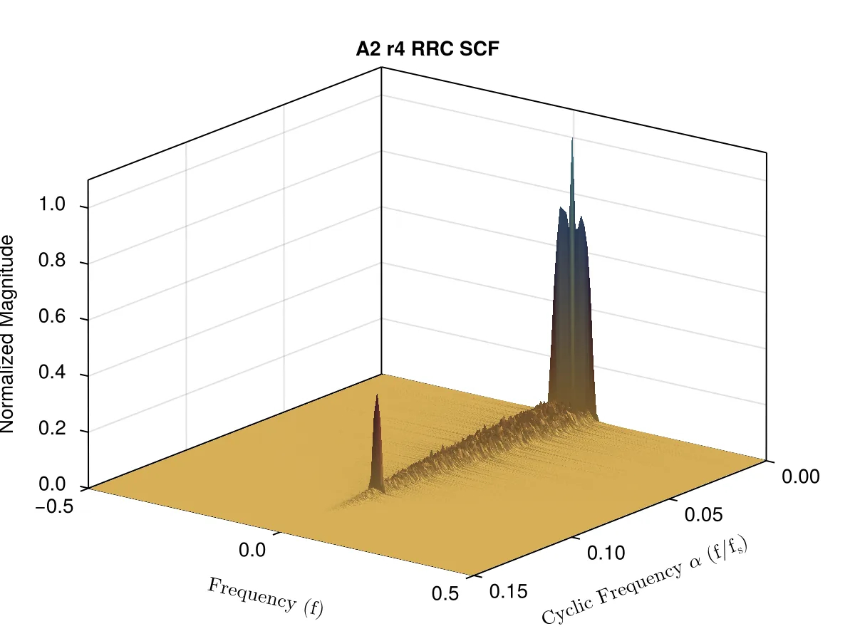
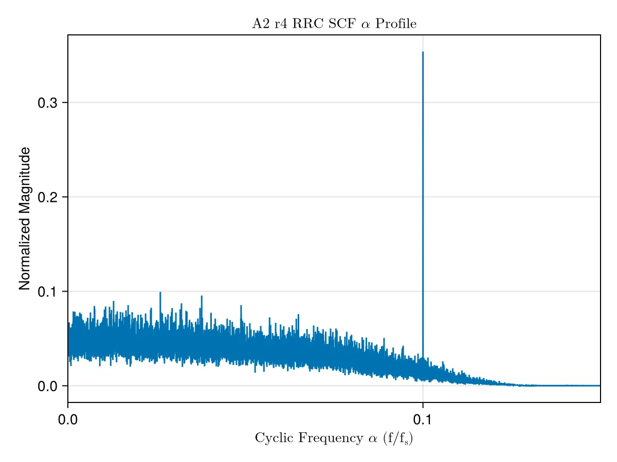
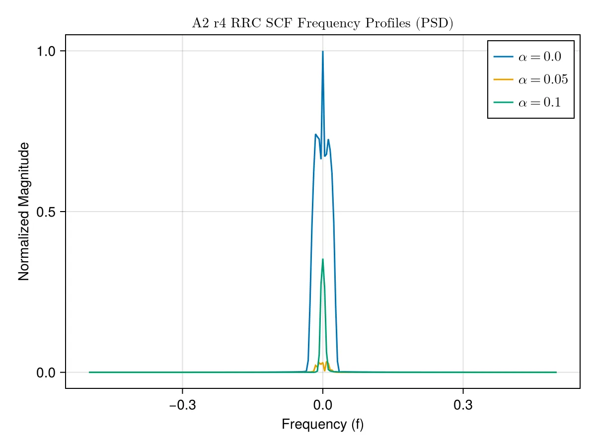
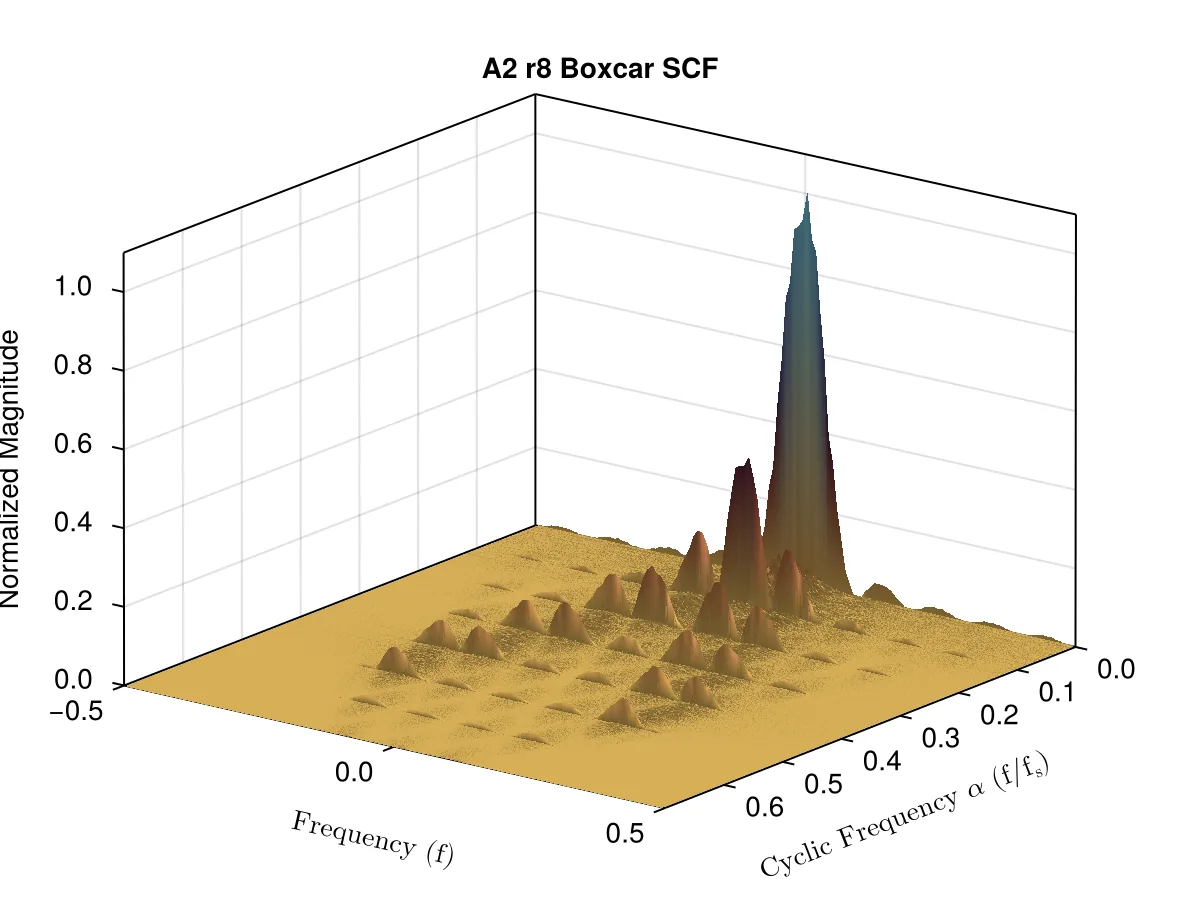
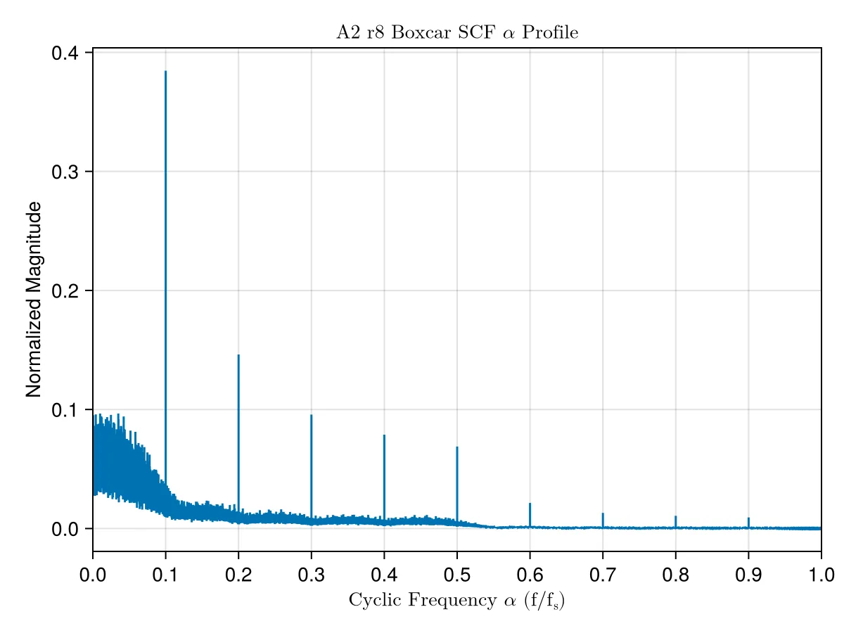
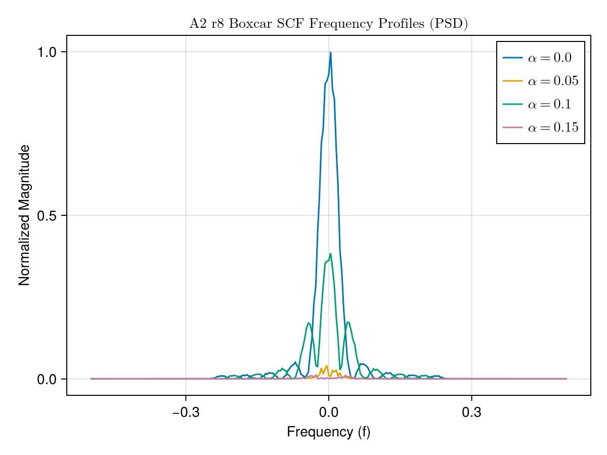
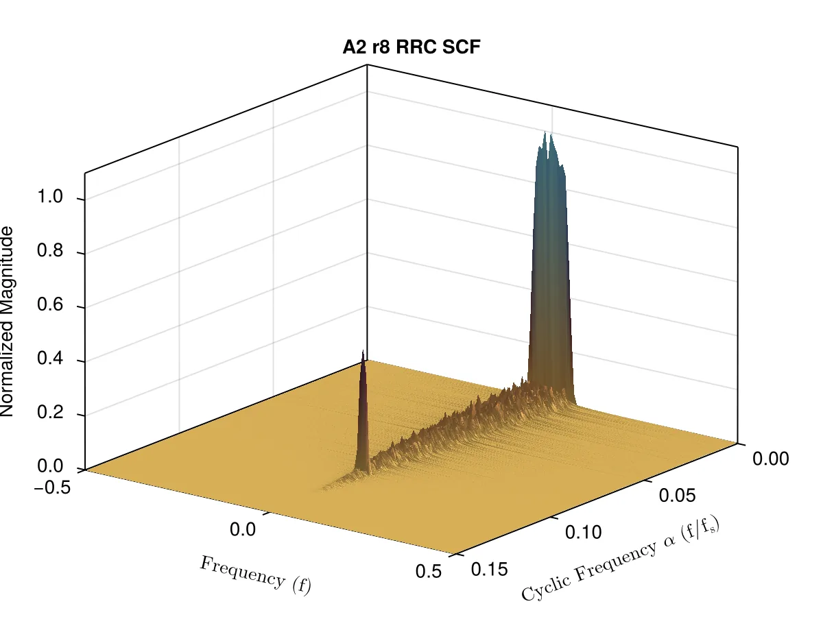
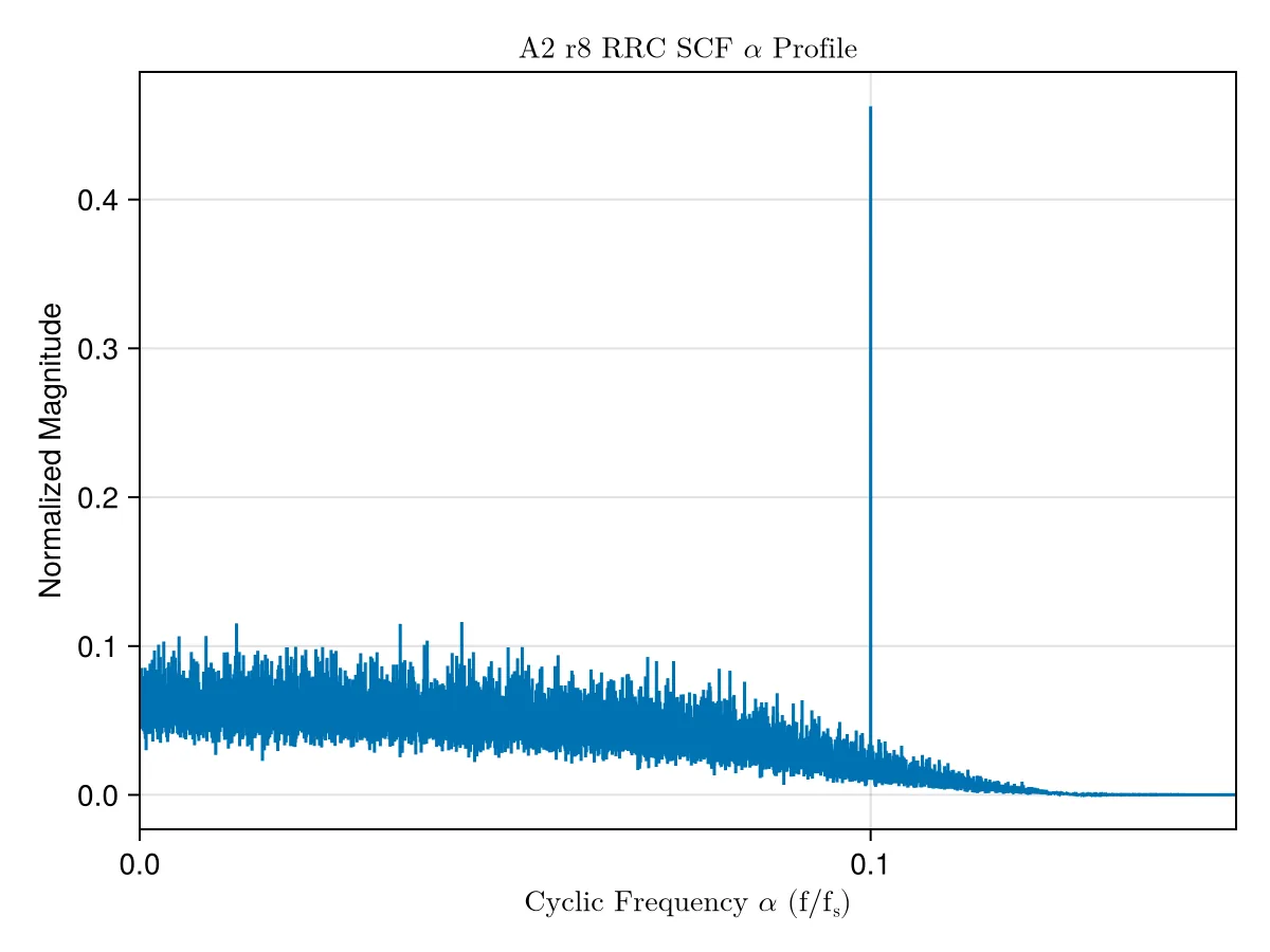
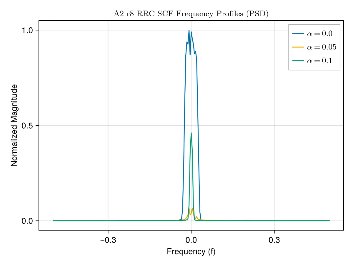
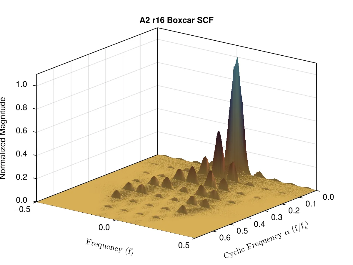
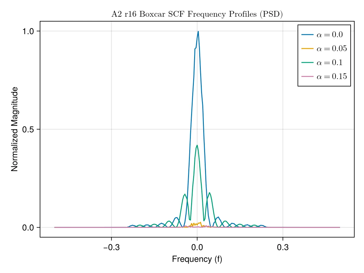
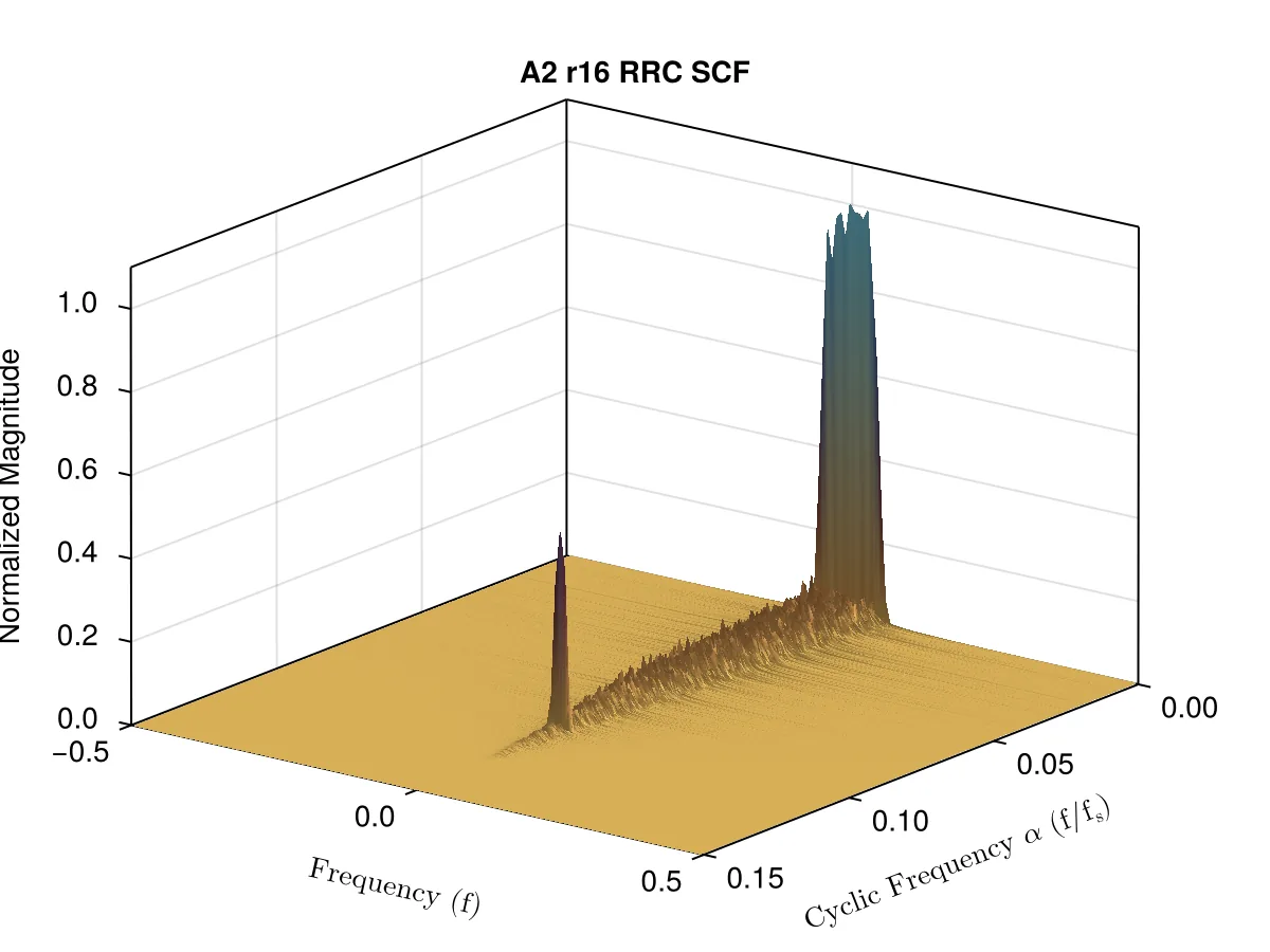
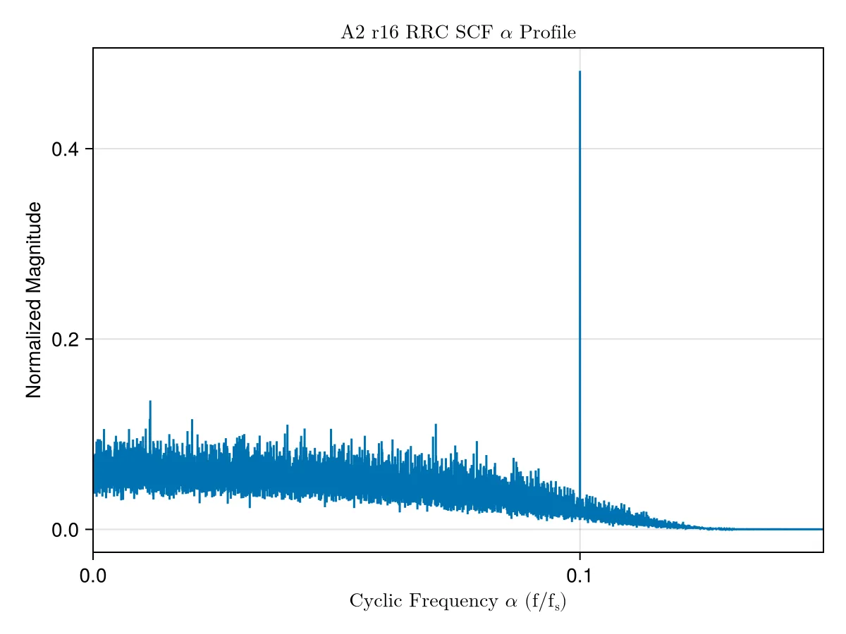
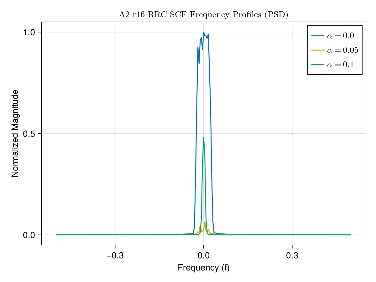
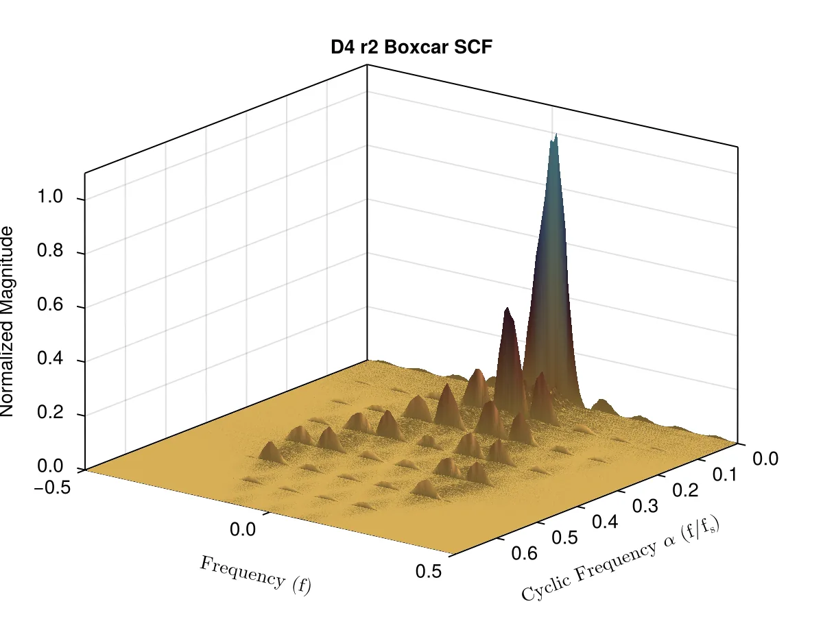
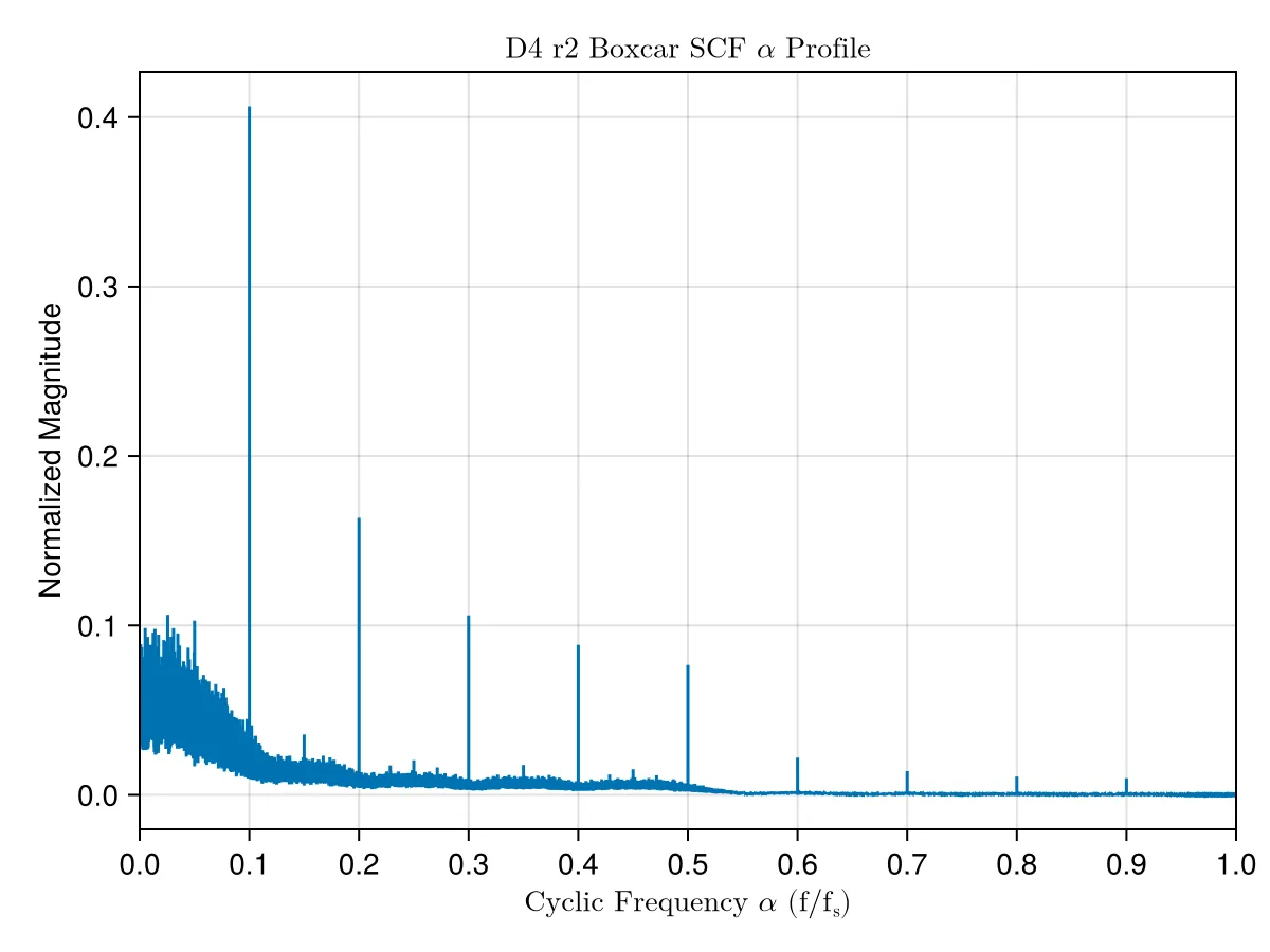
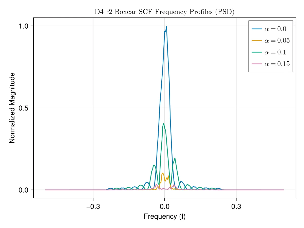
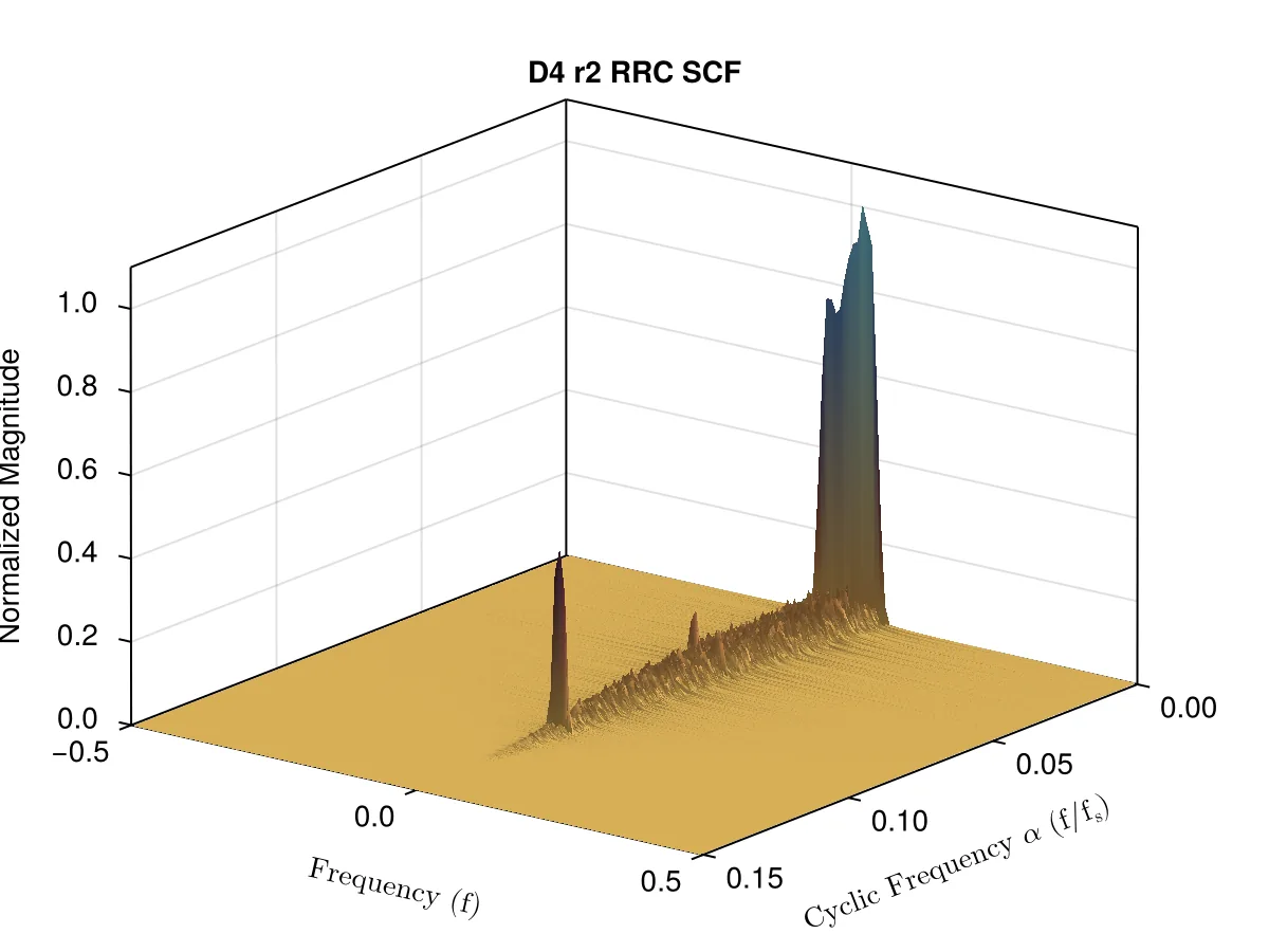
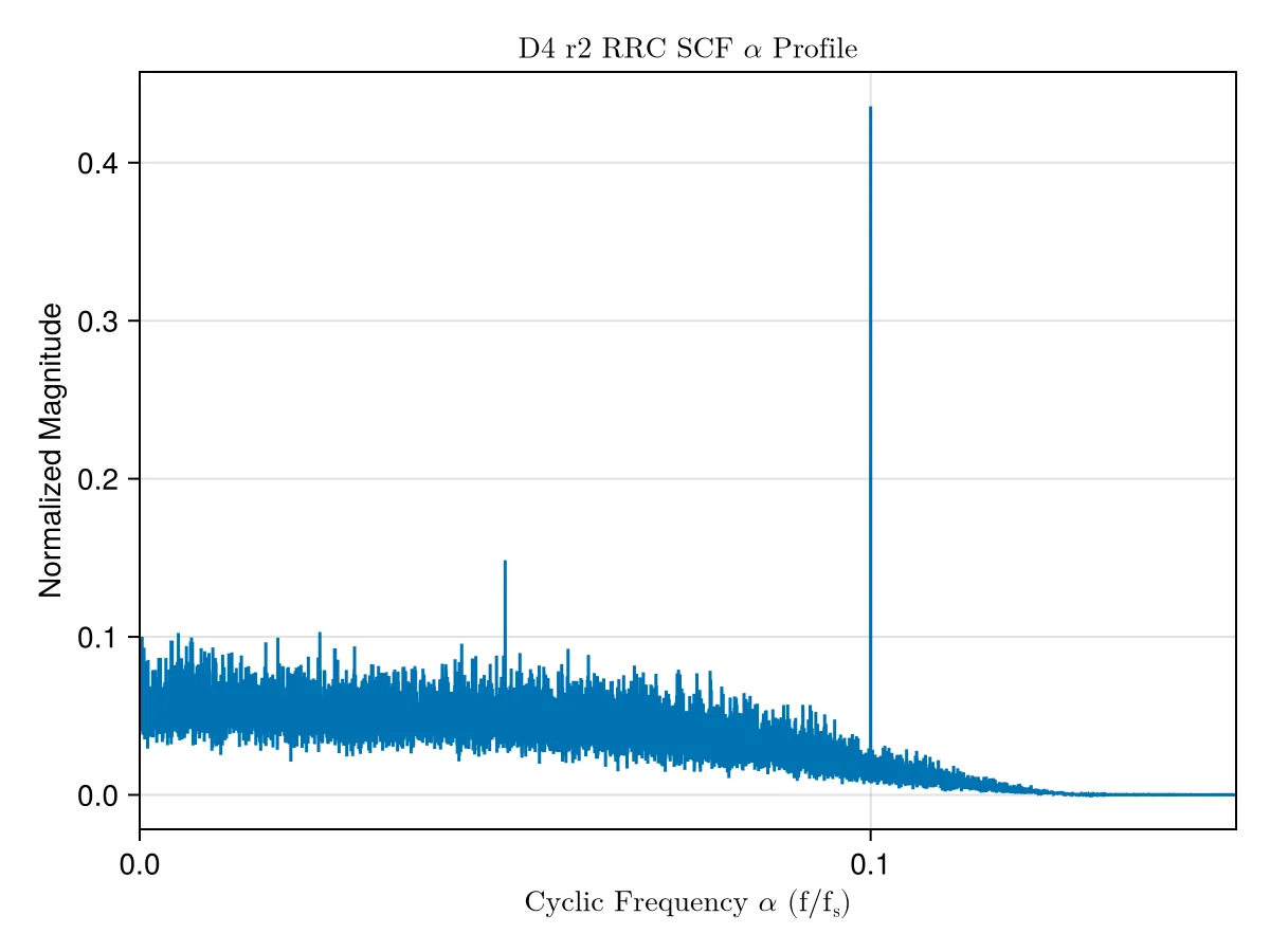
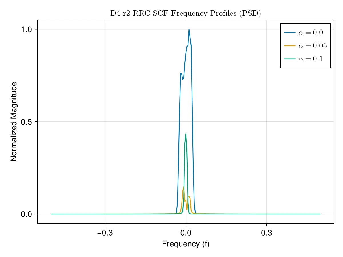
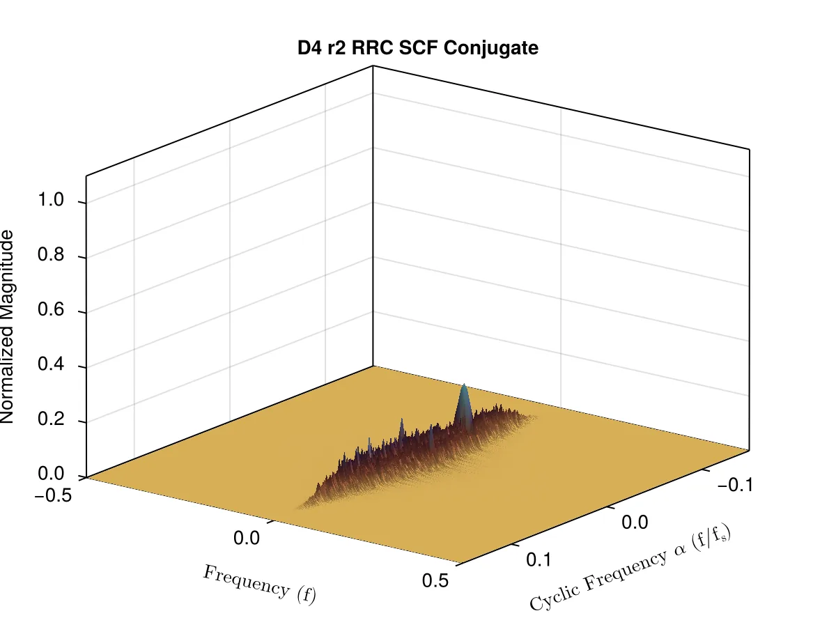
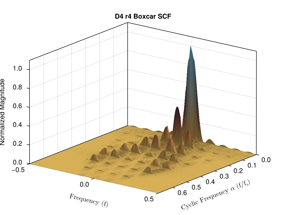
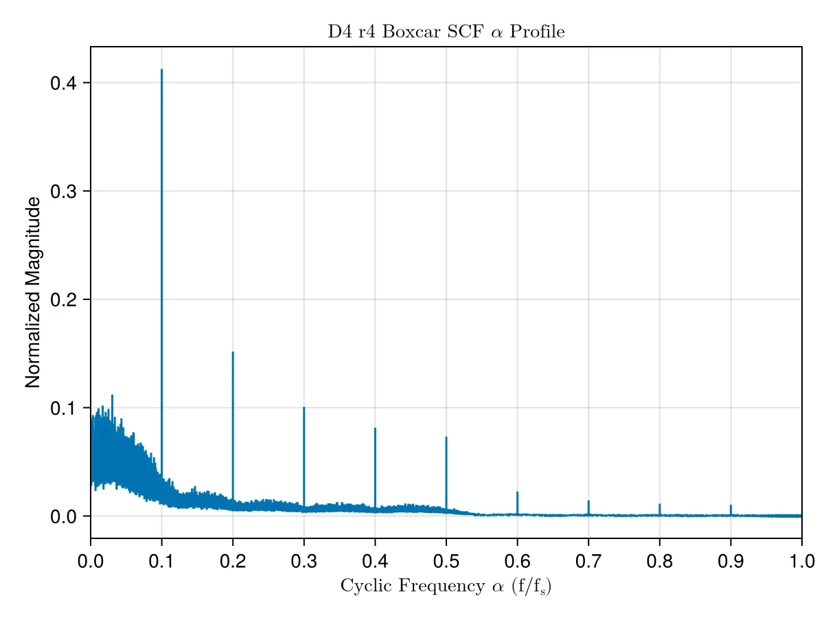
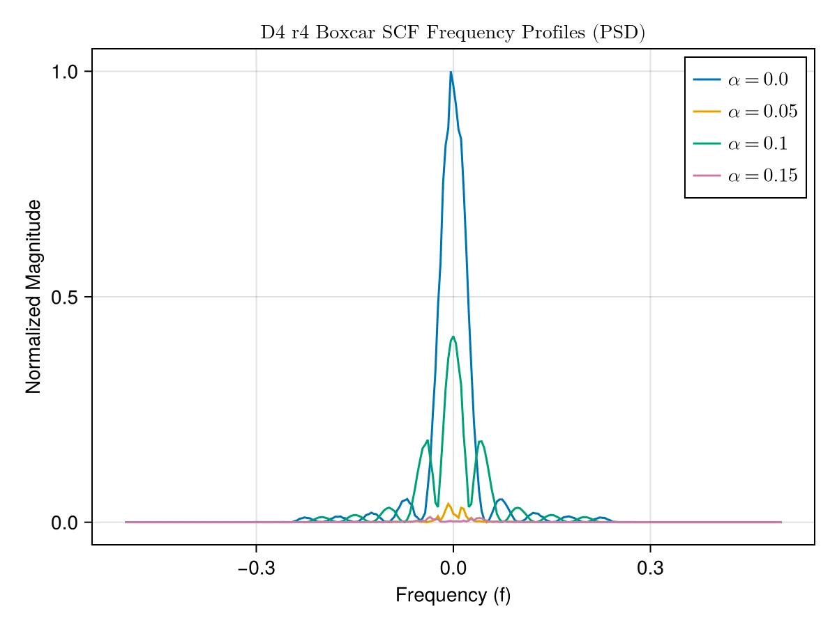
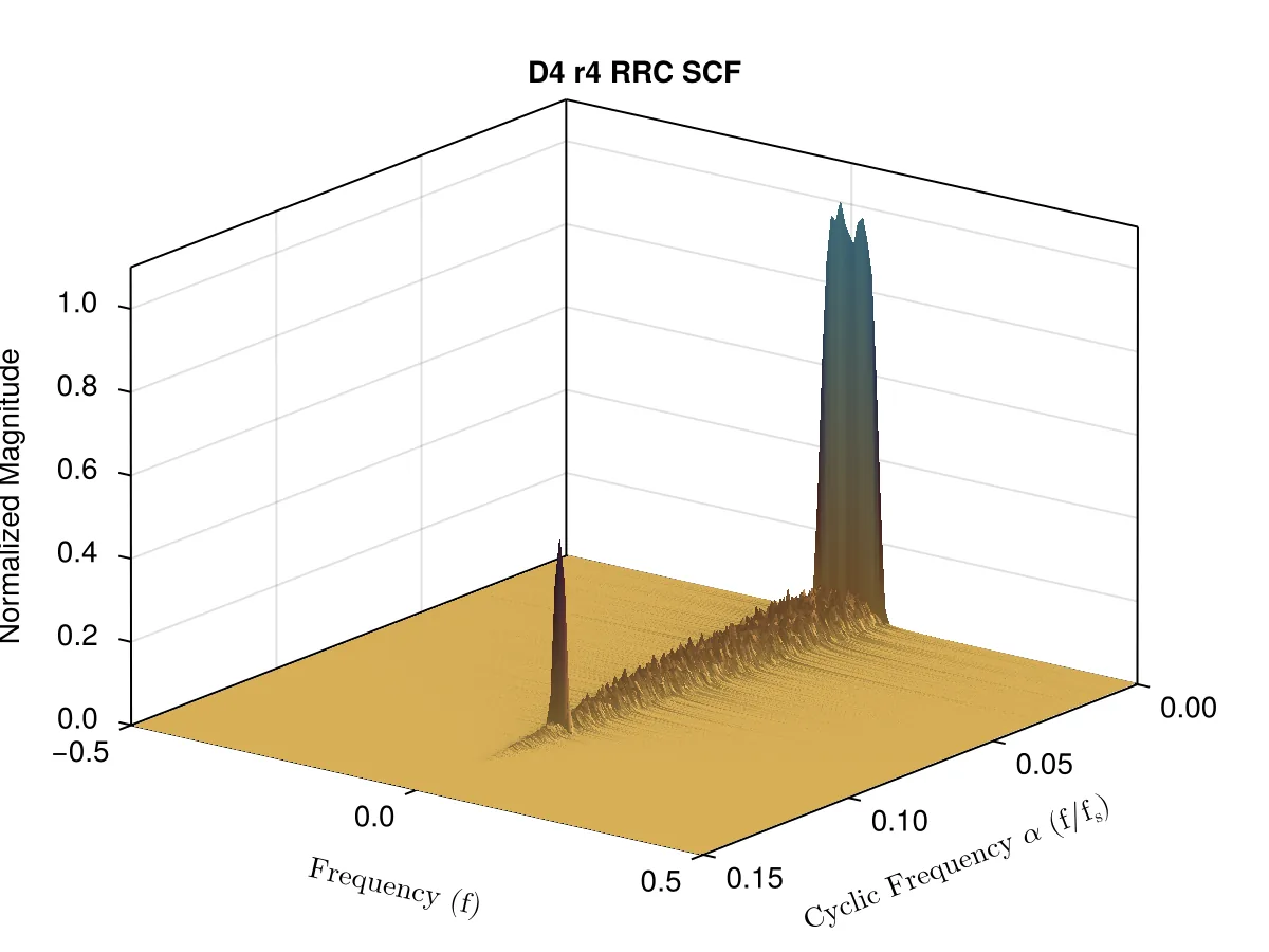
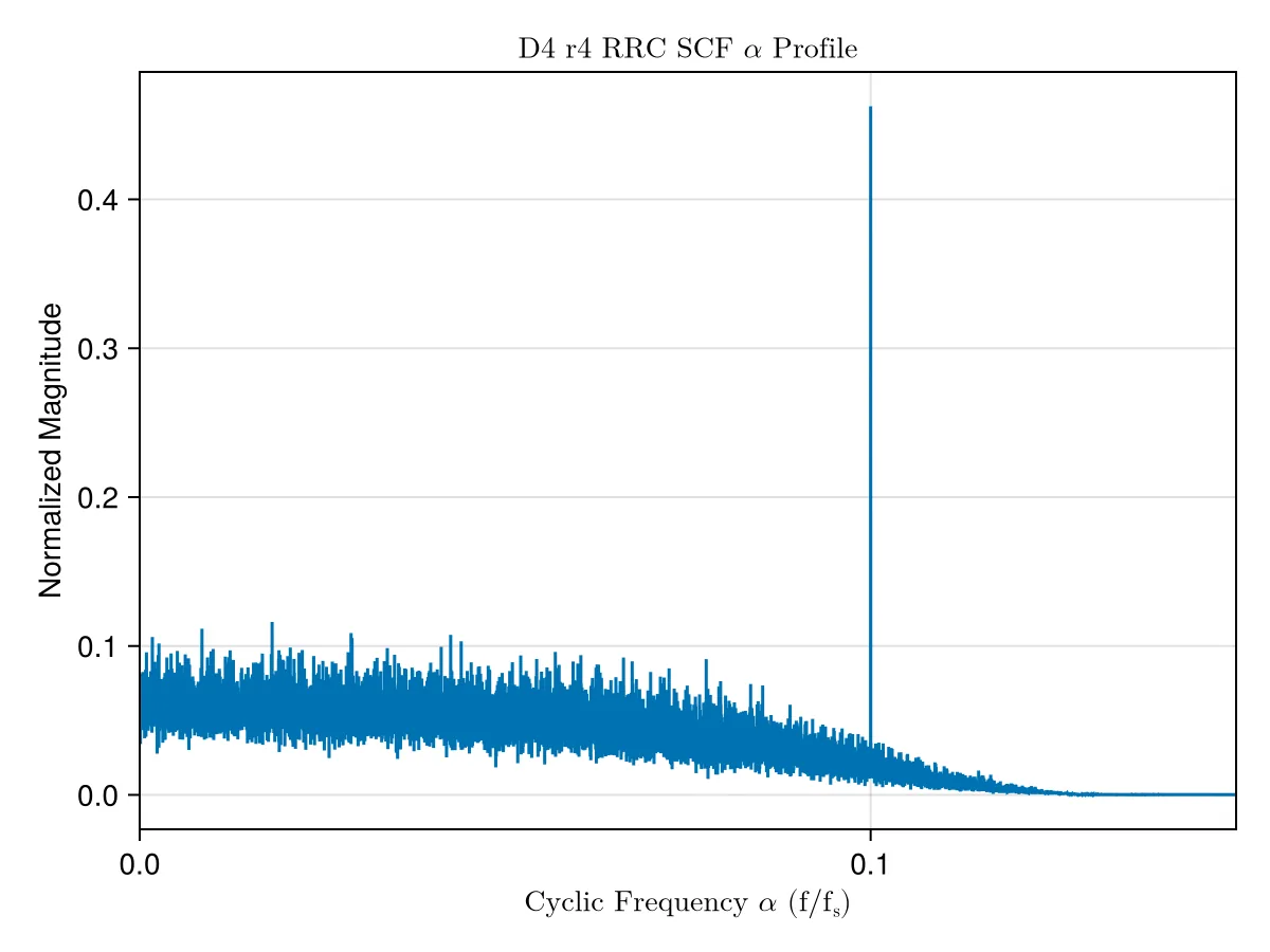
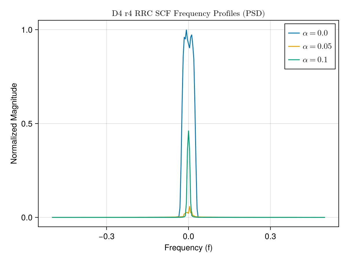
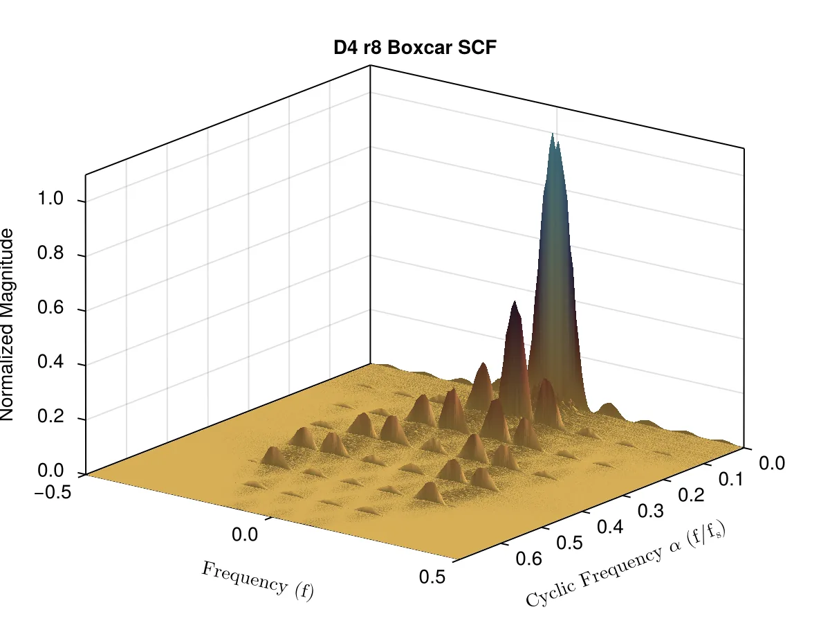
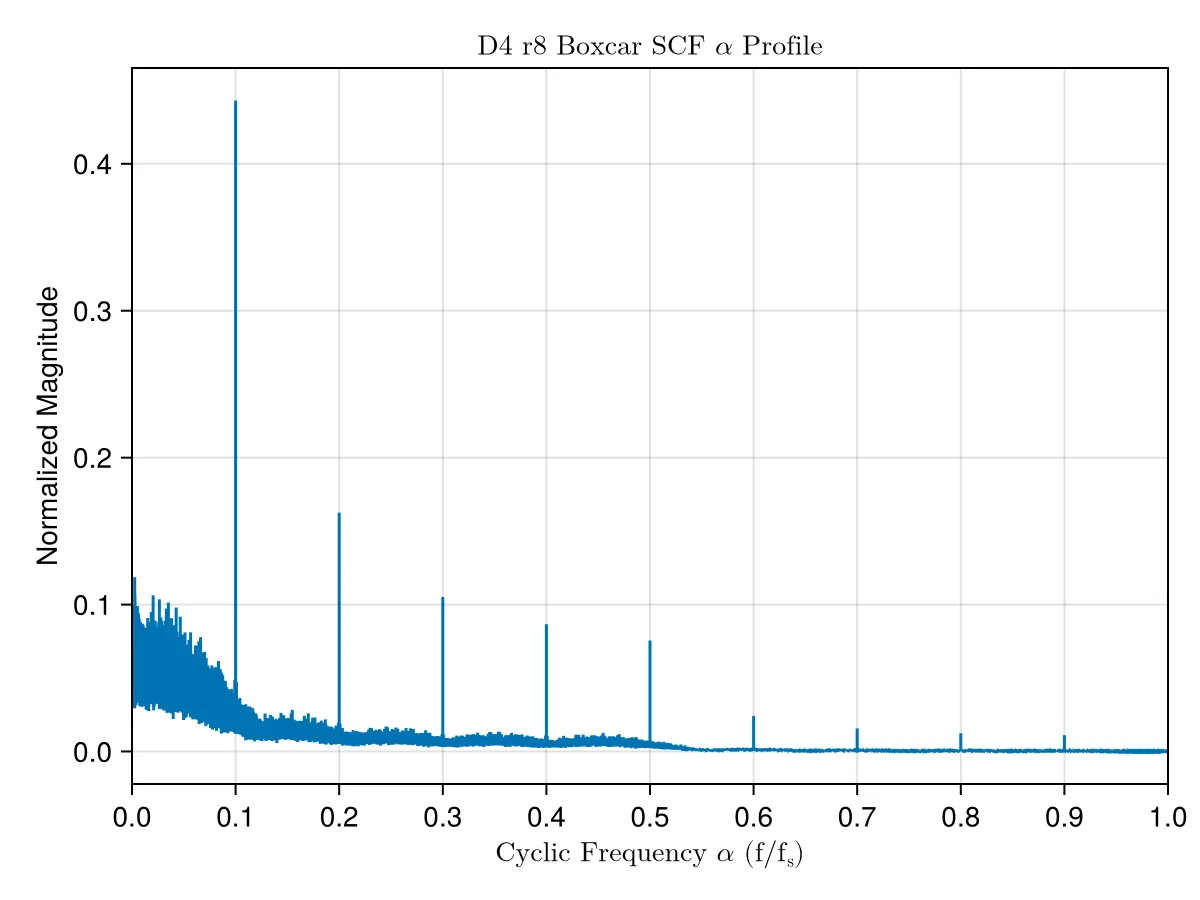
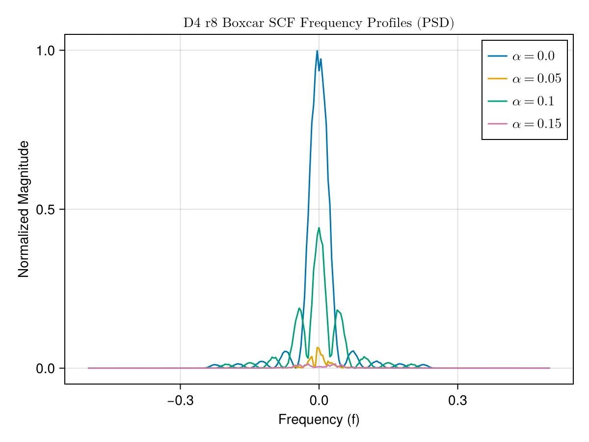
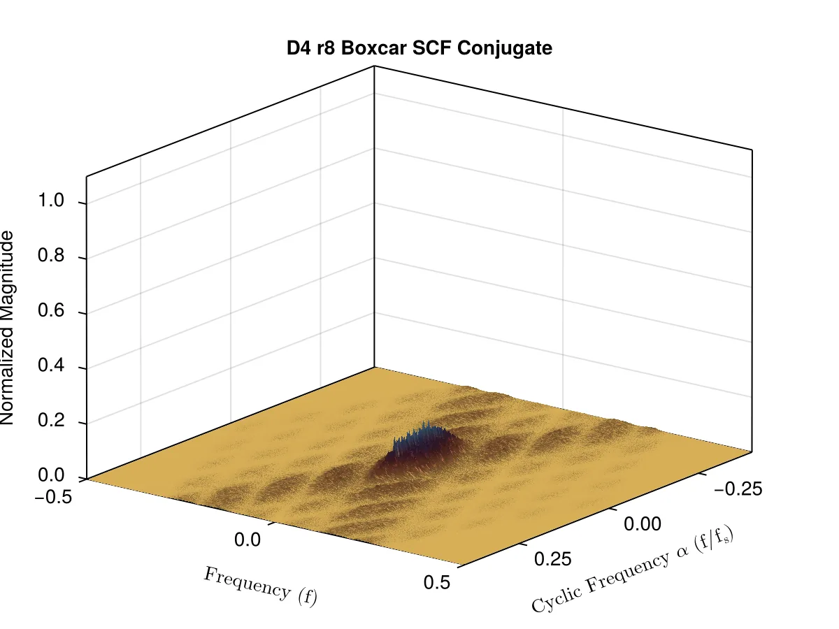
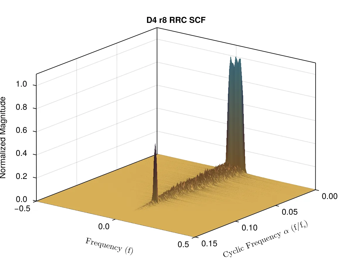
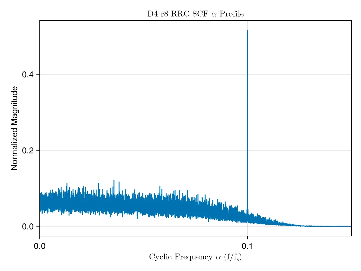
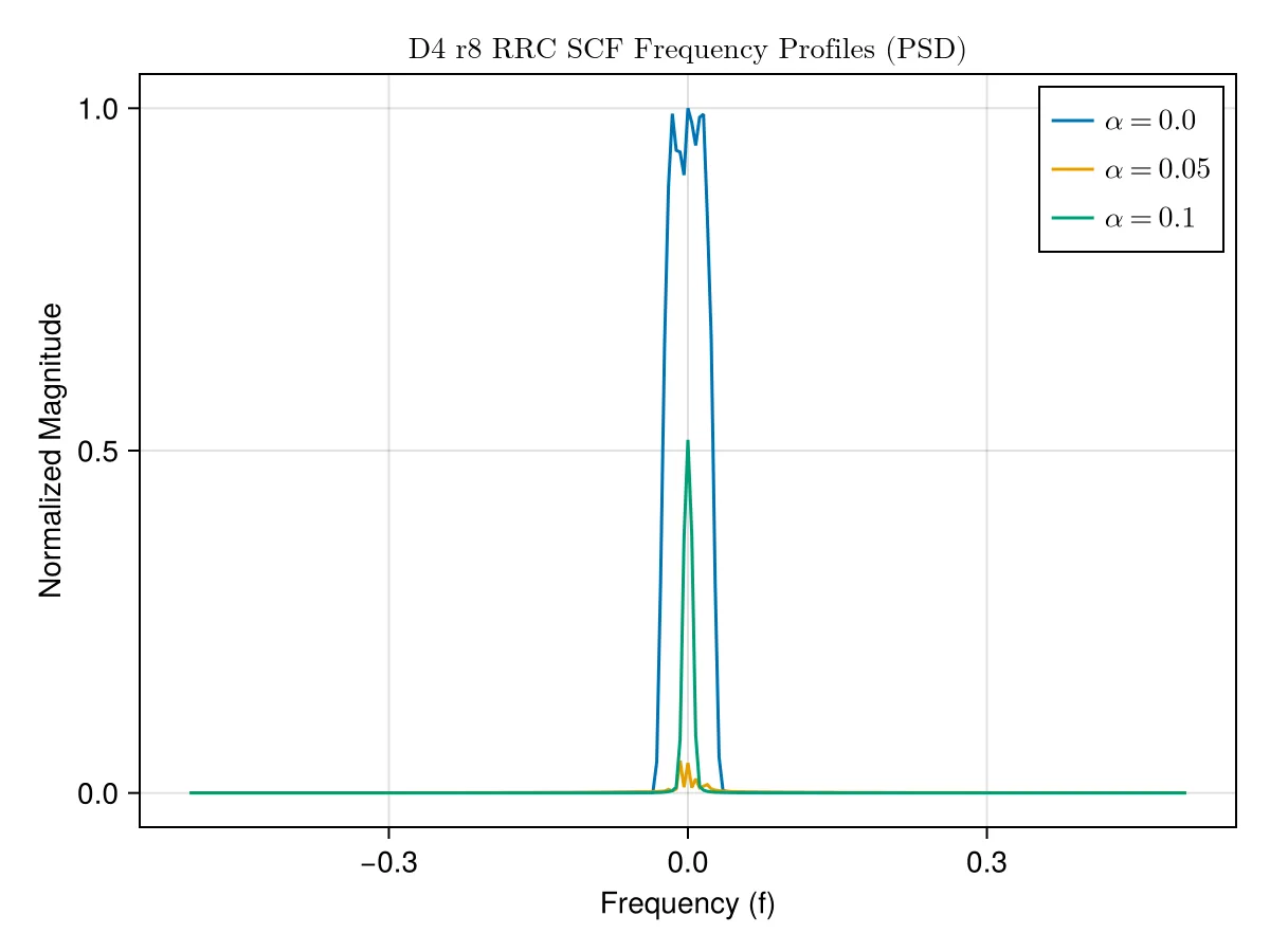
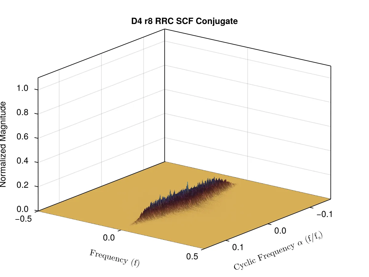
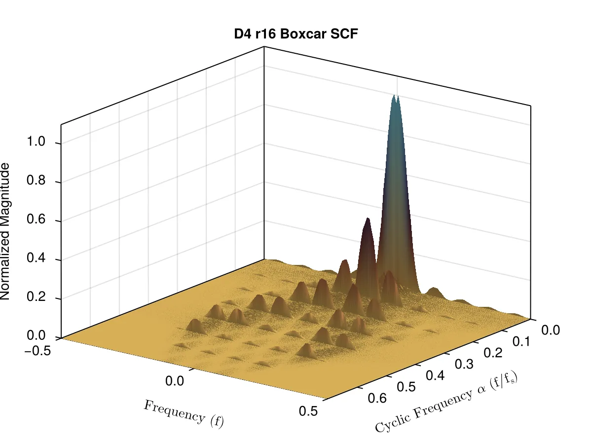
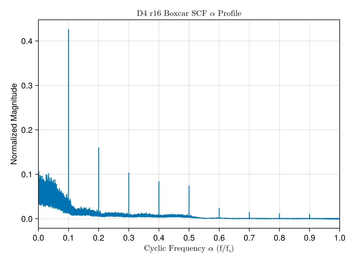
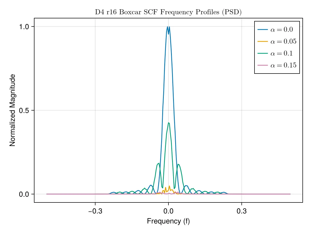
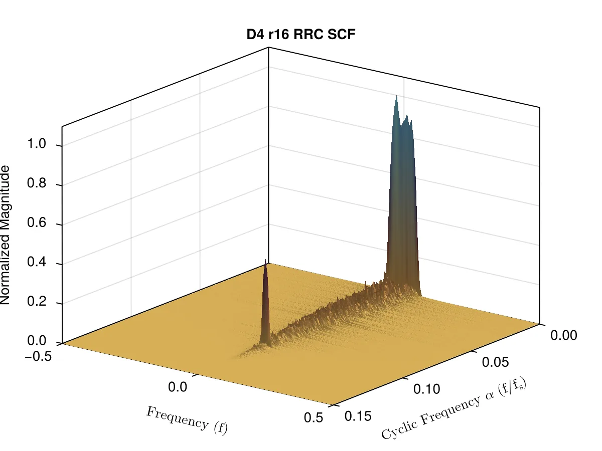
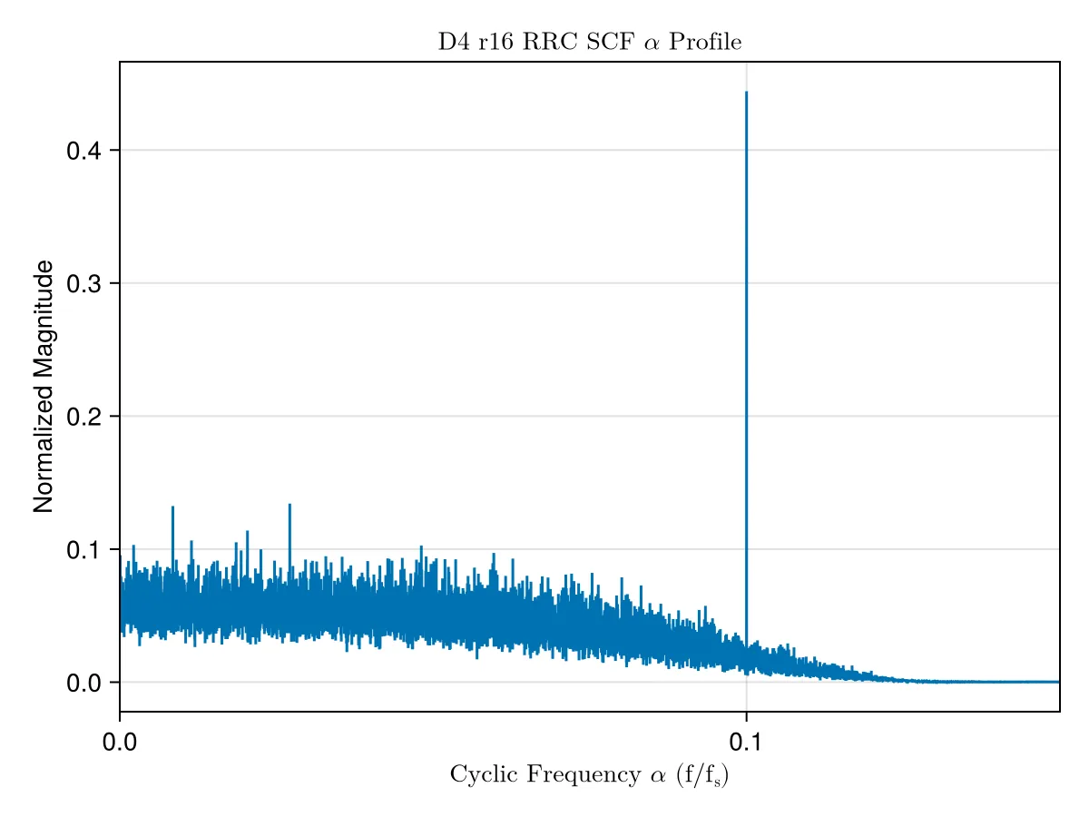
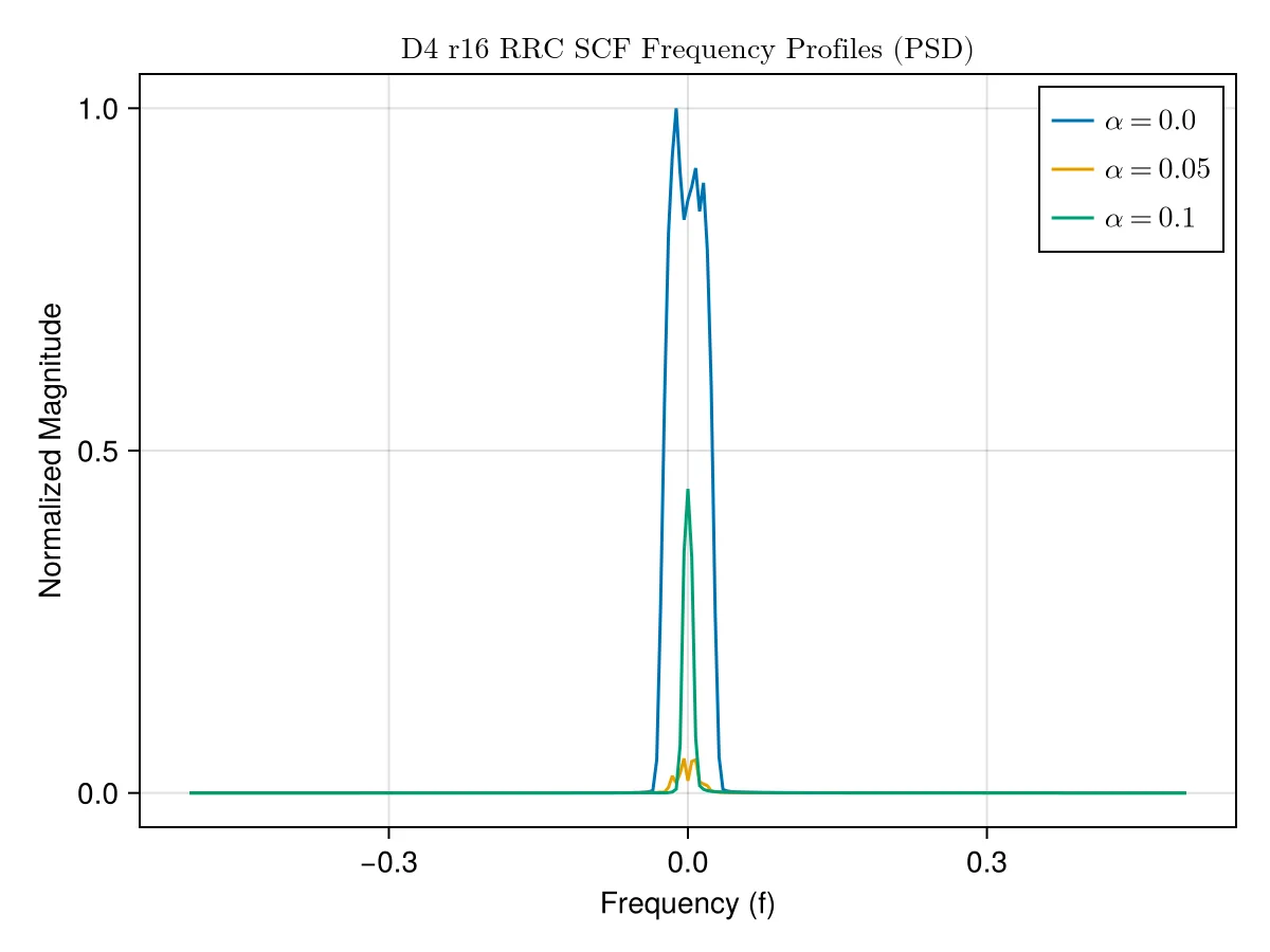
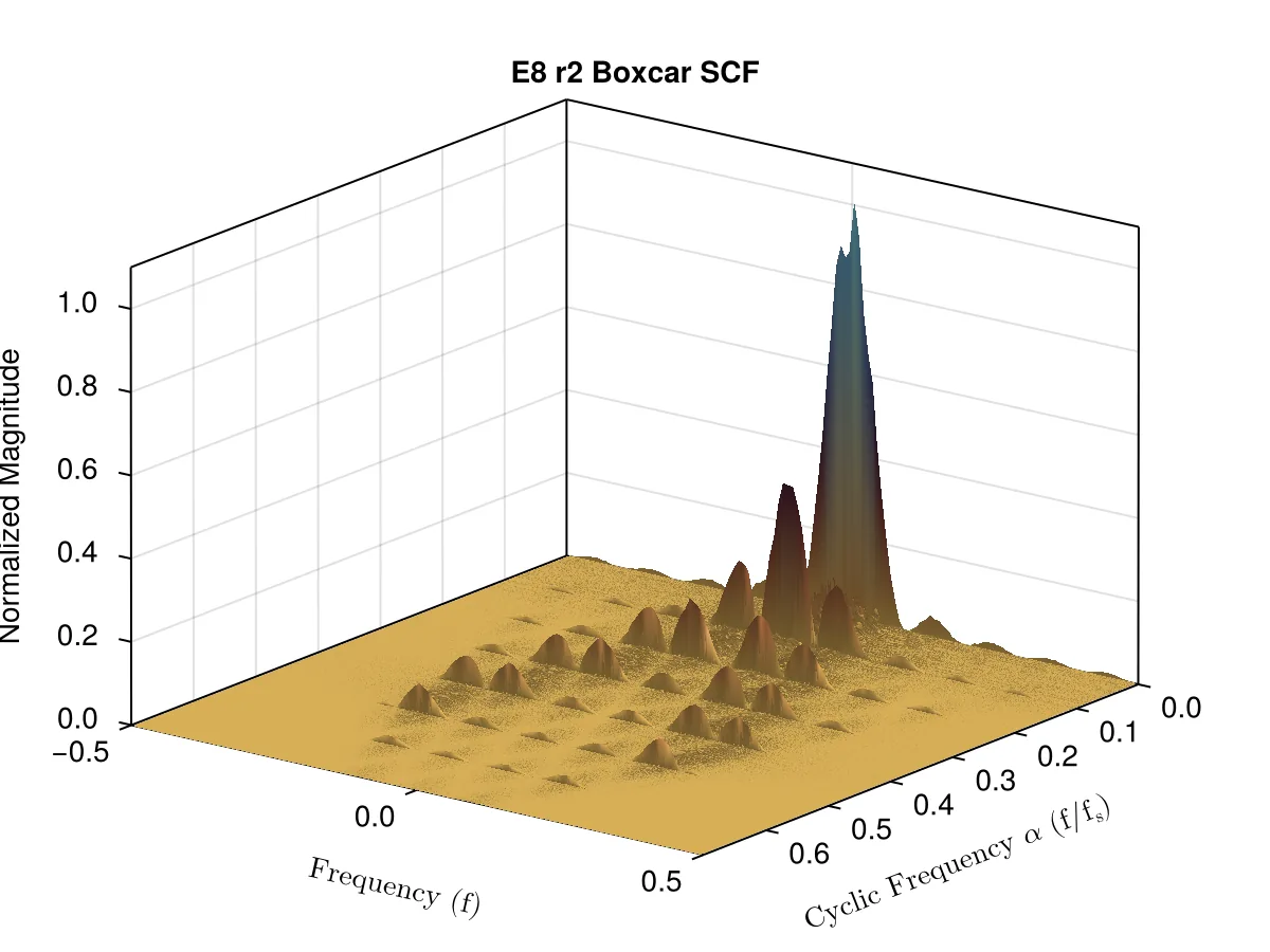
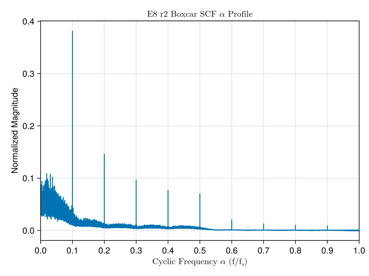
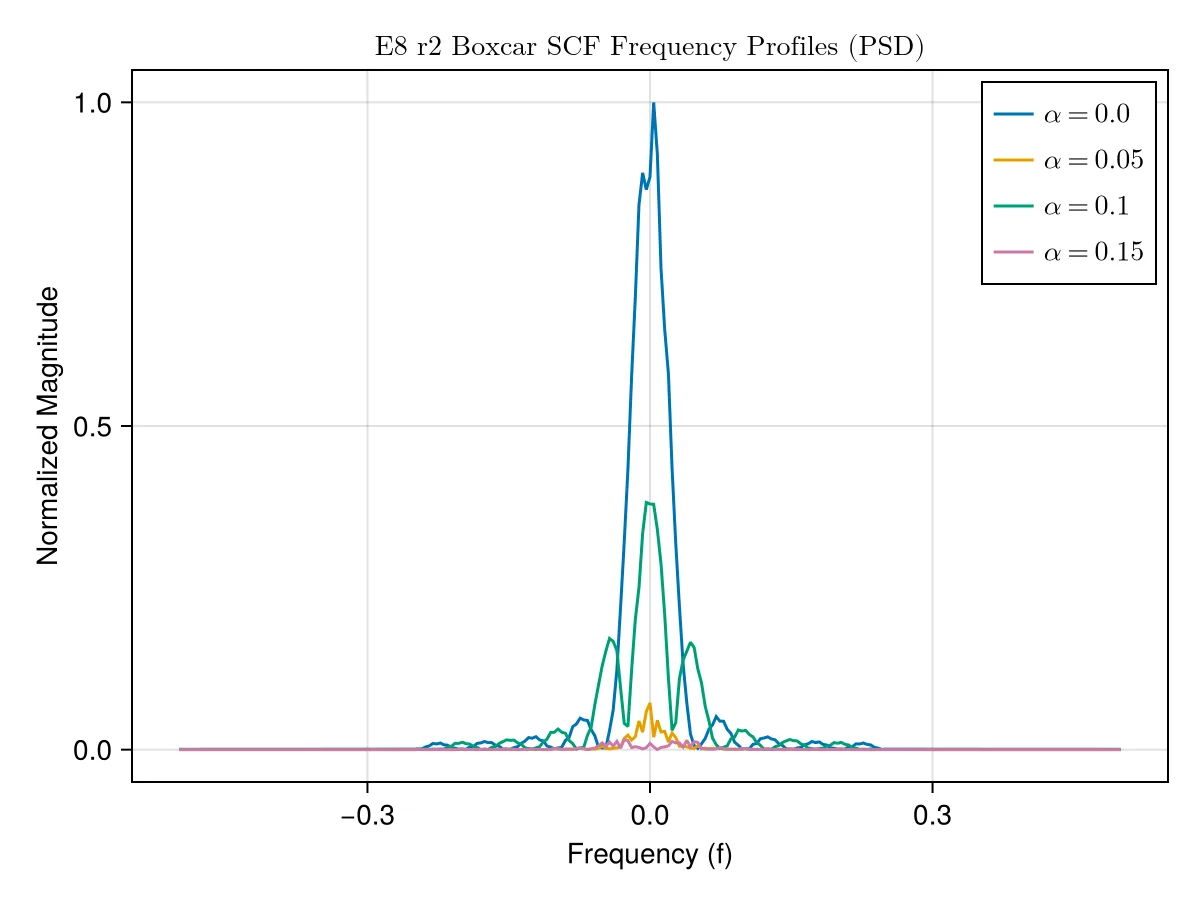
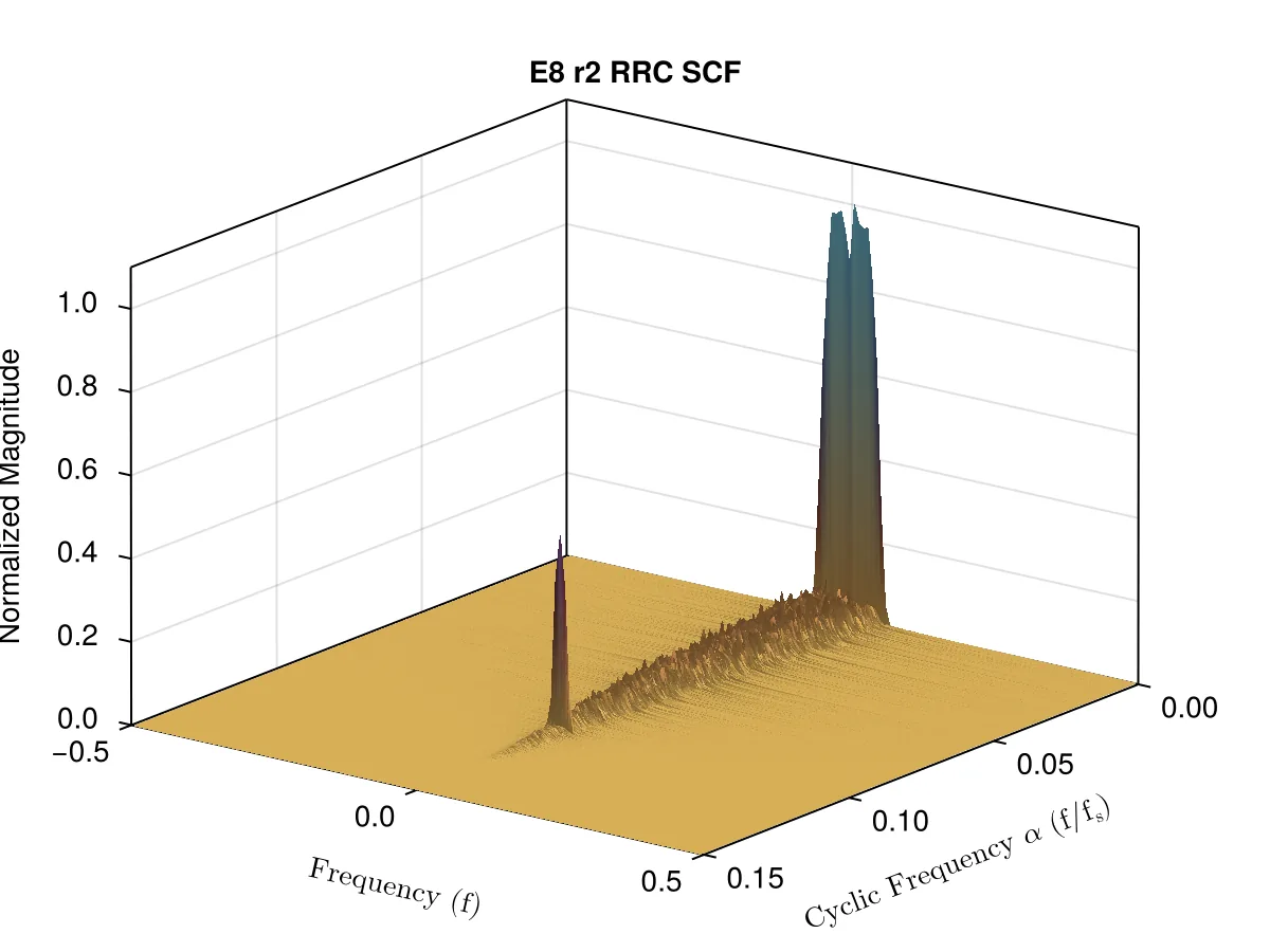
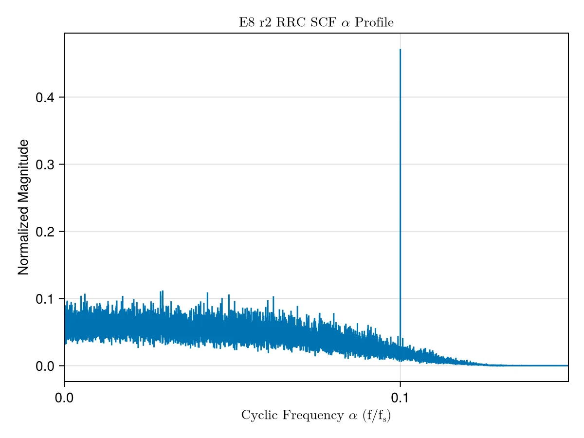
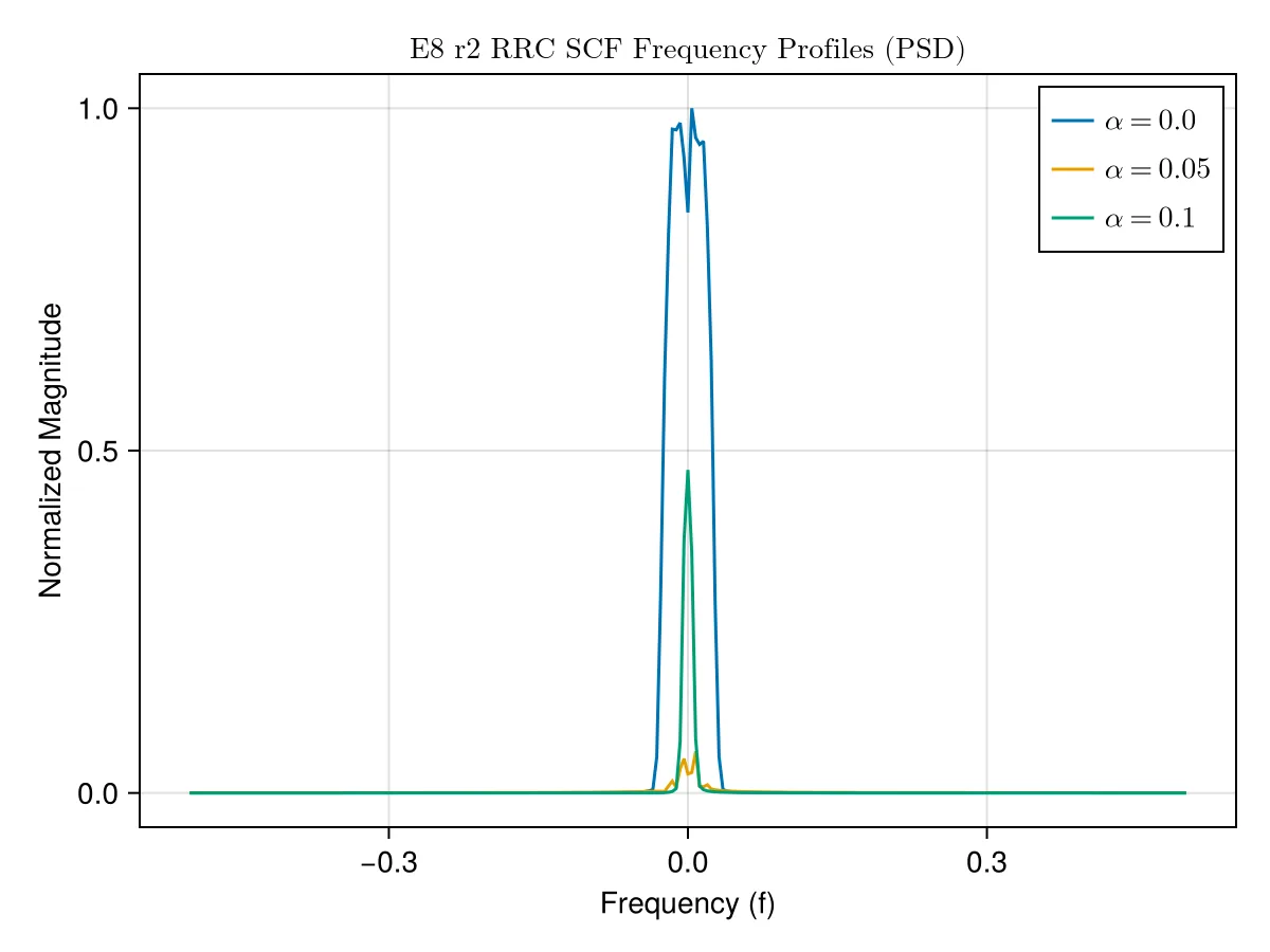
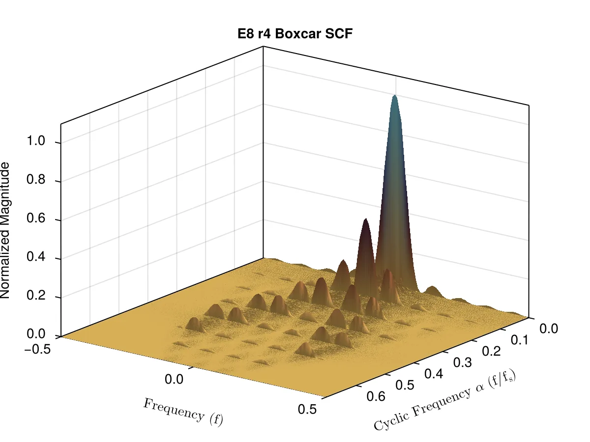
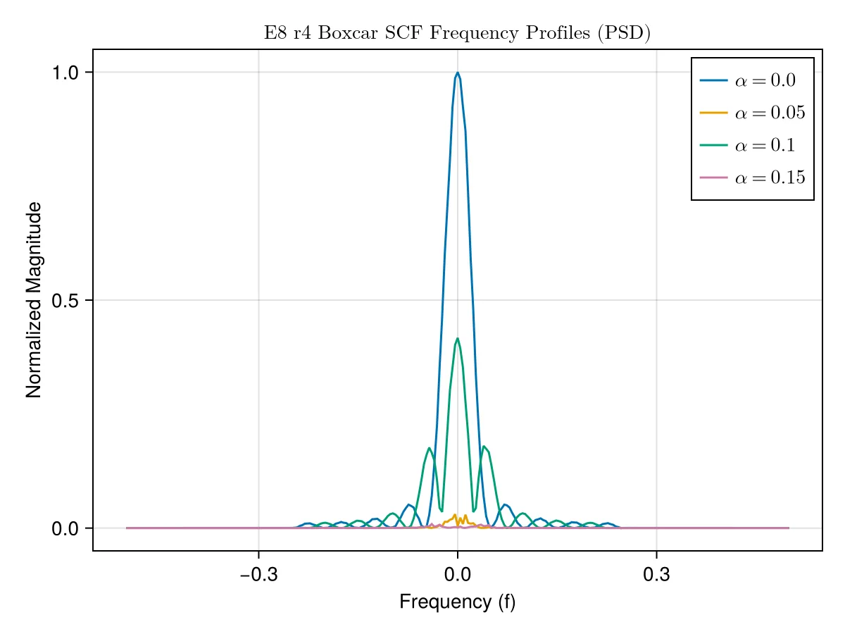
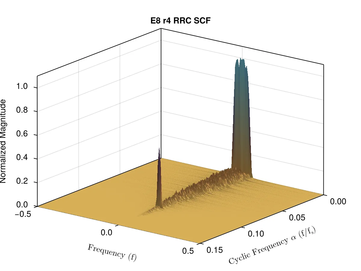
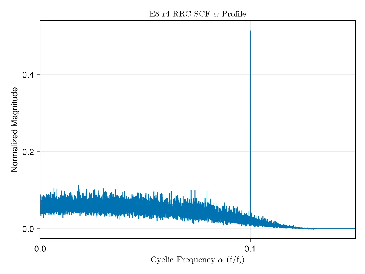
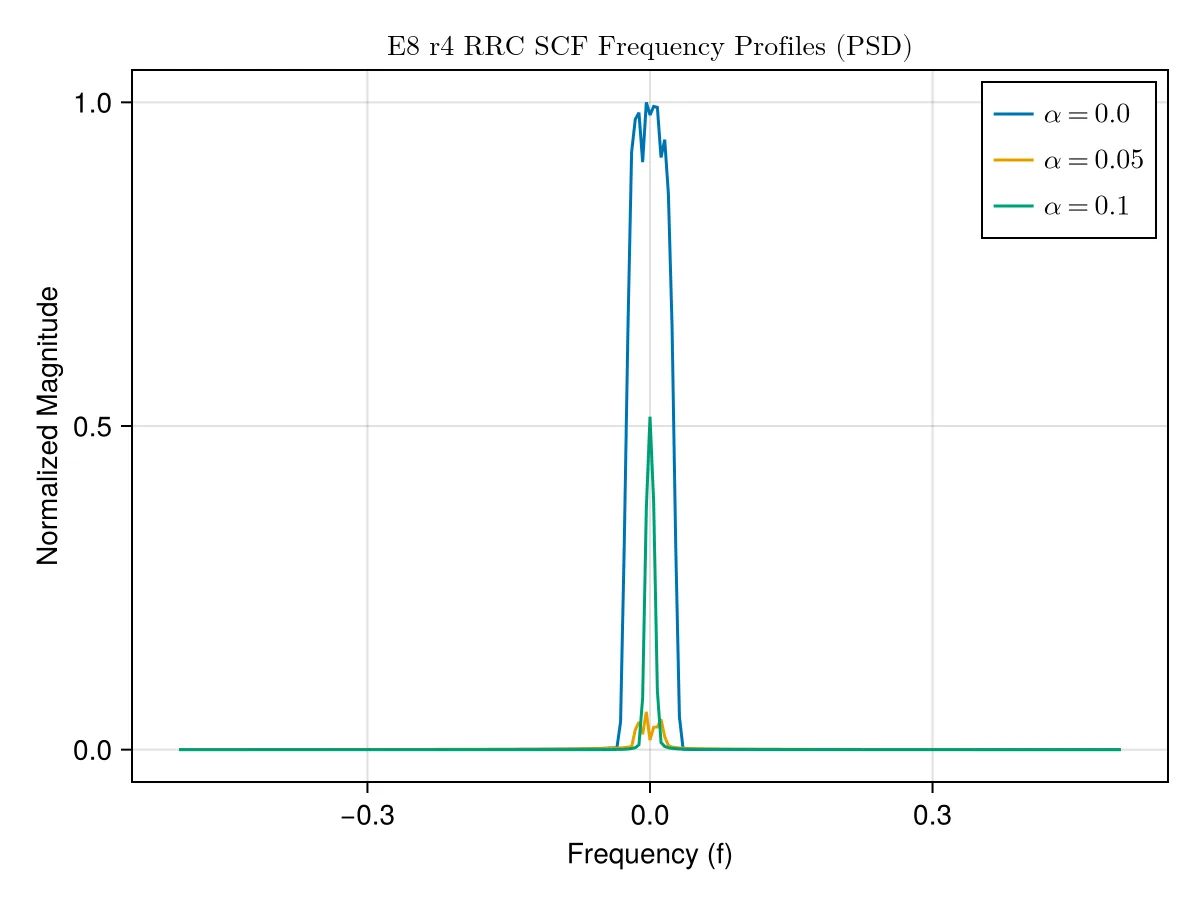
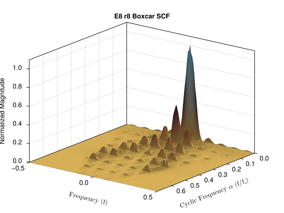
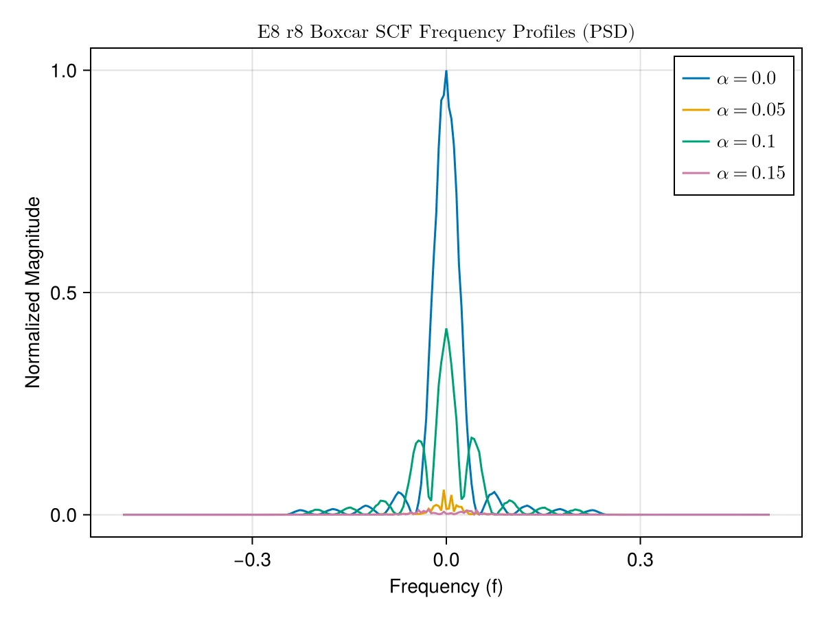
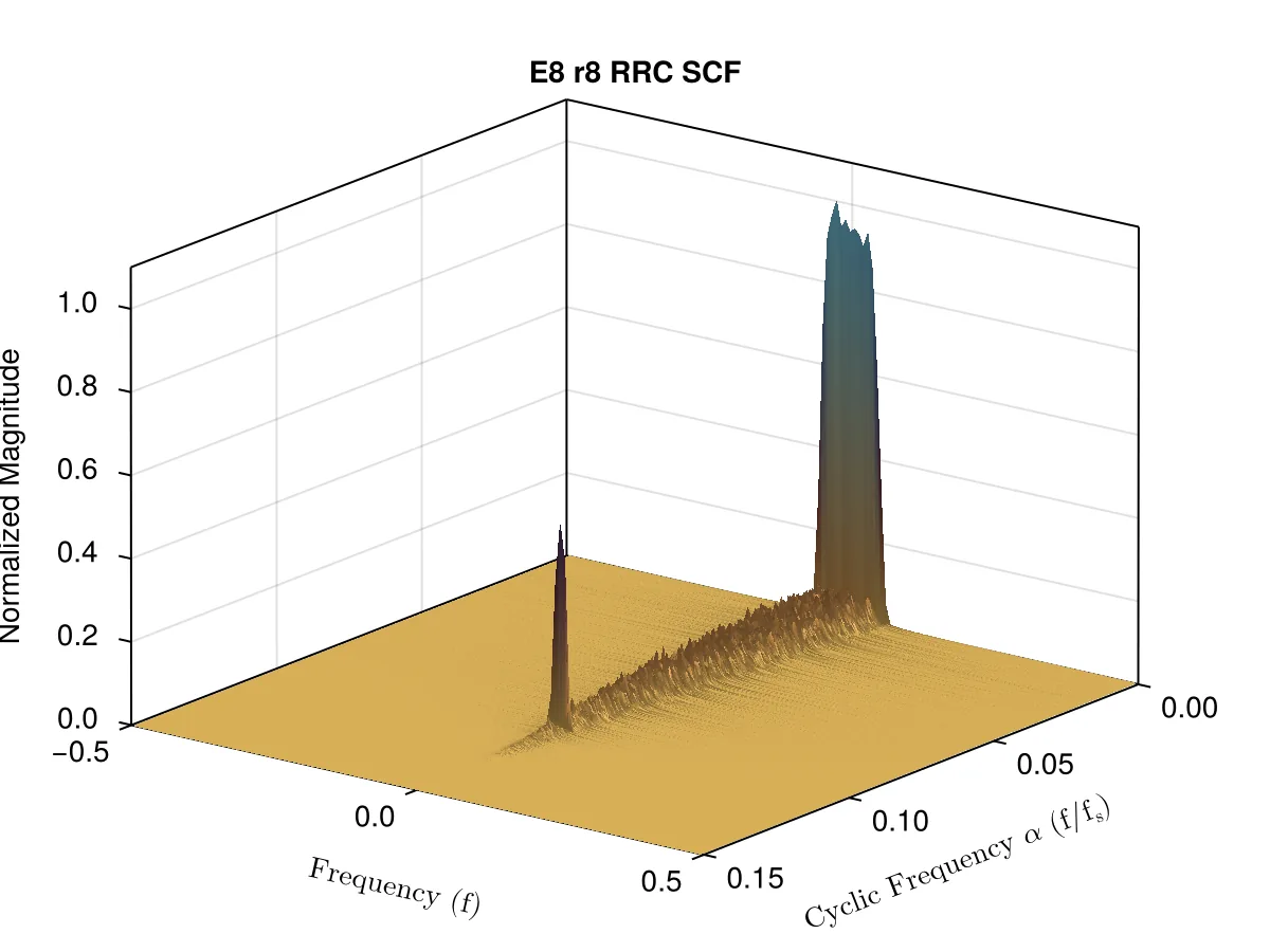
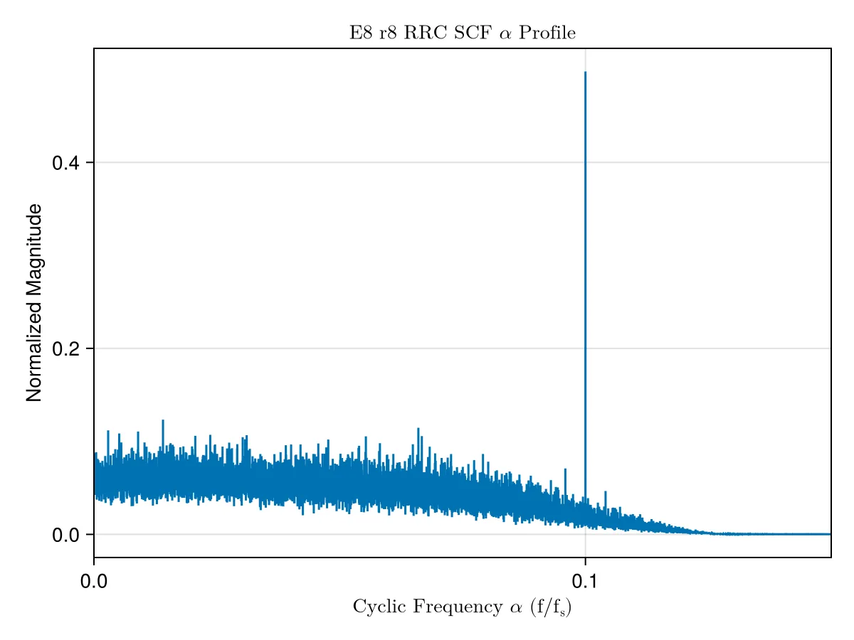
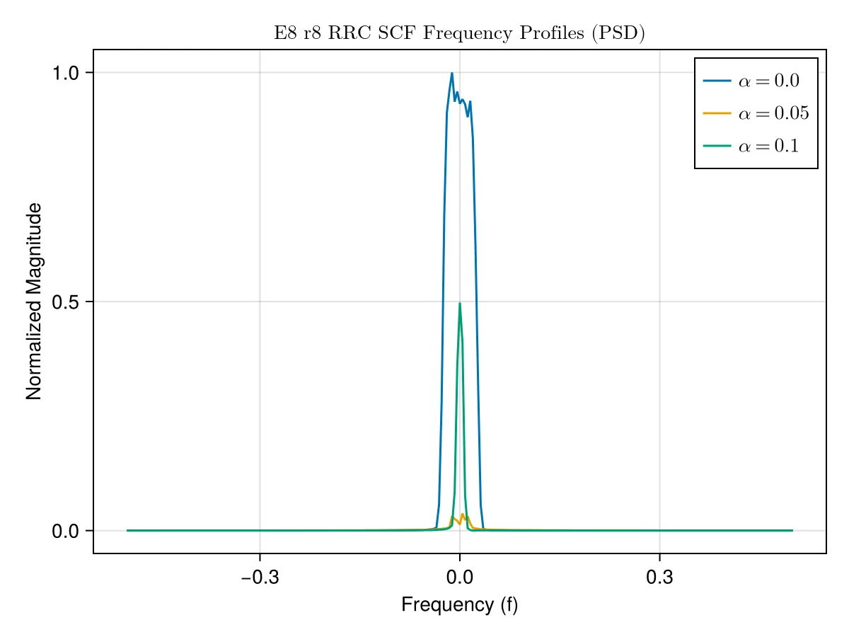
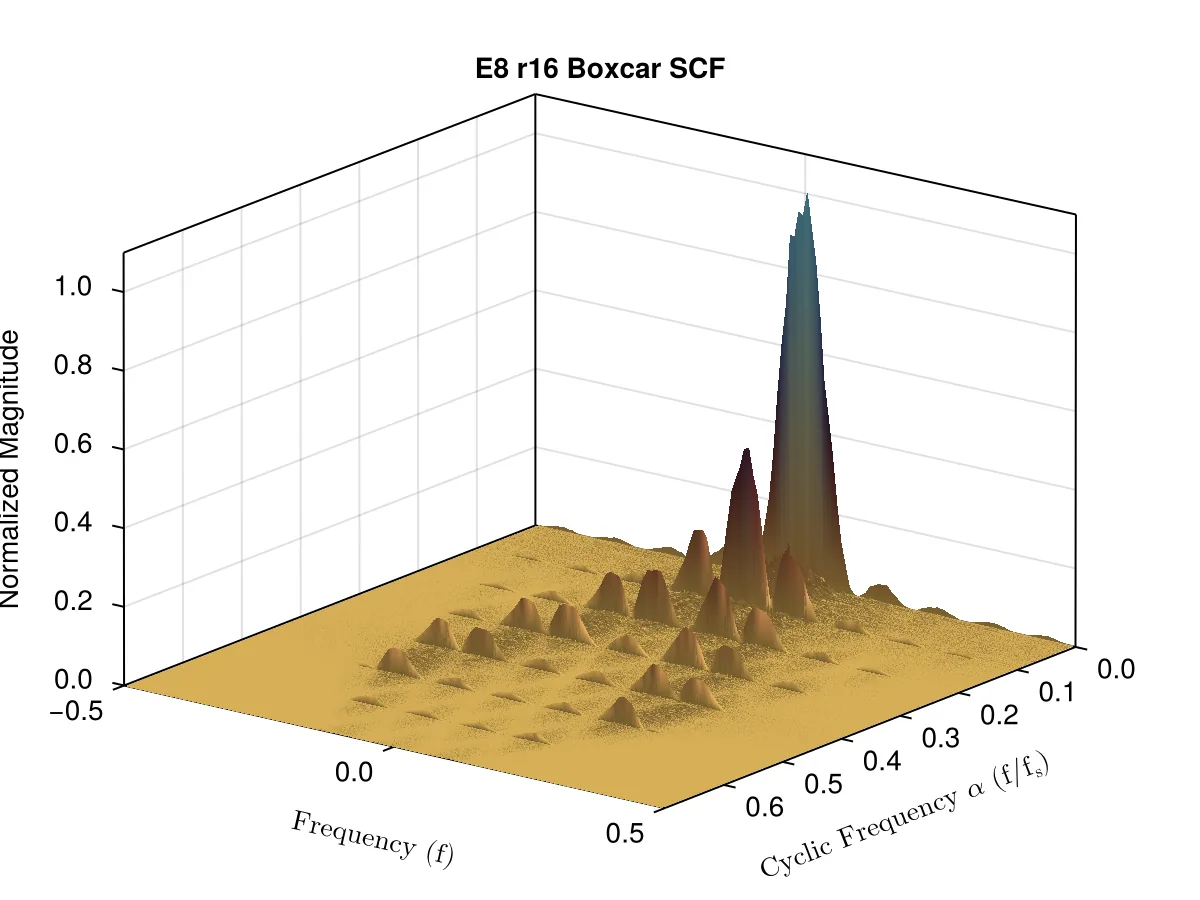
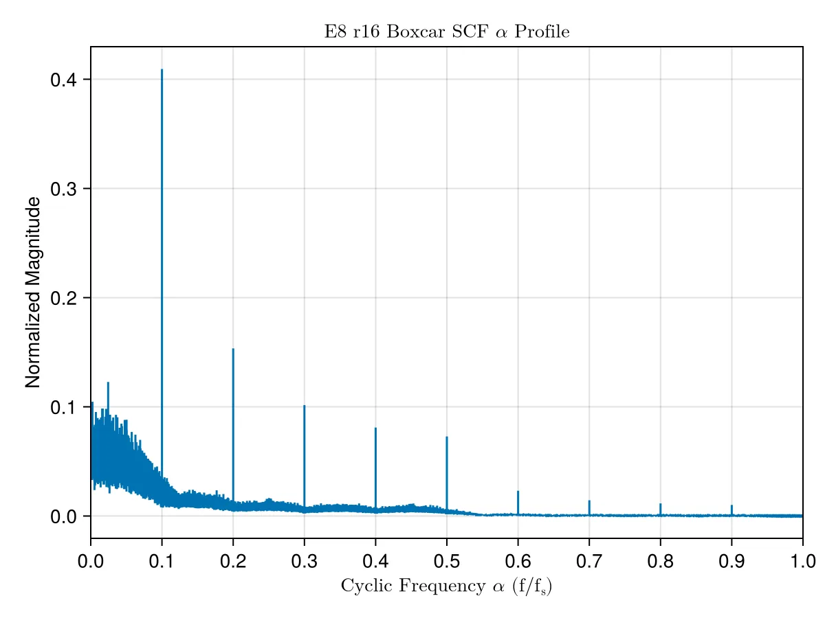
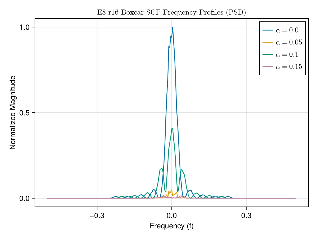
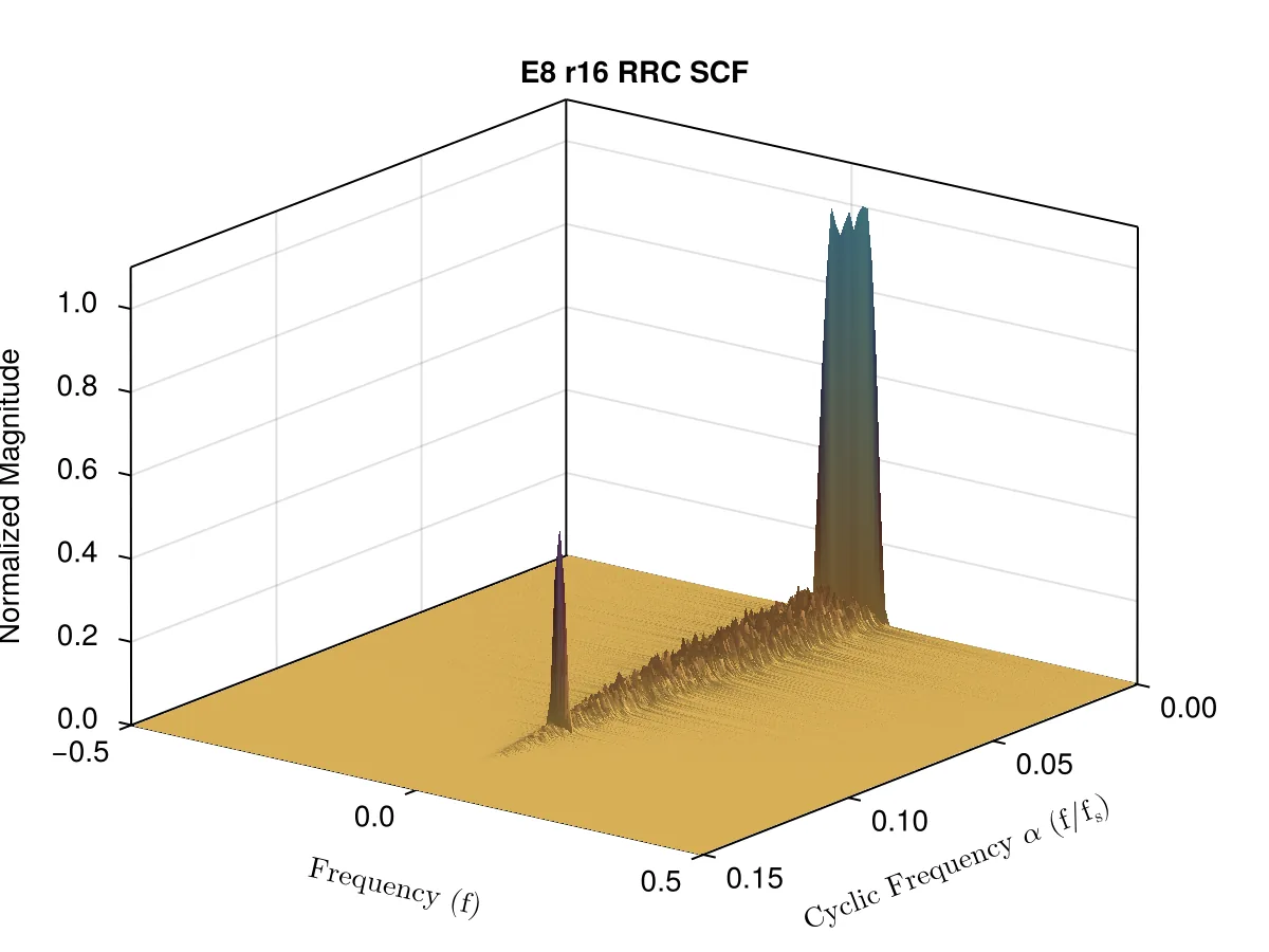
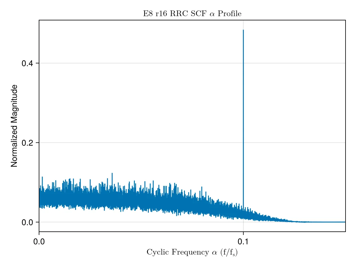
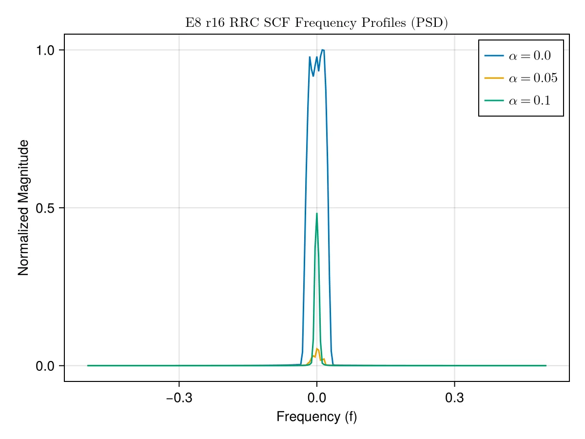
The Spectral Correlation Function, or SCF, shows the correlation between two different frequency components. The CAF and the SCF show similar components, with CAF in the time domain and SCF in the frequency domain. The alpha profile still spikes at 1/(symbol rate) while the base of the spike in the frequency-profile sports a width of 1/(symbol rate).

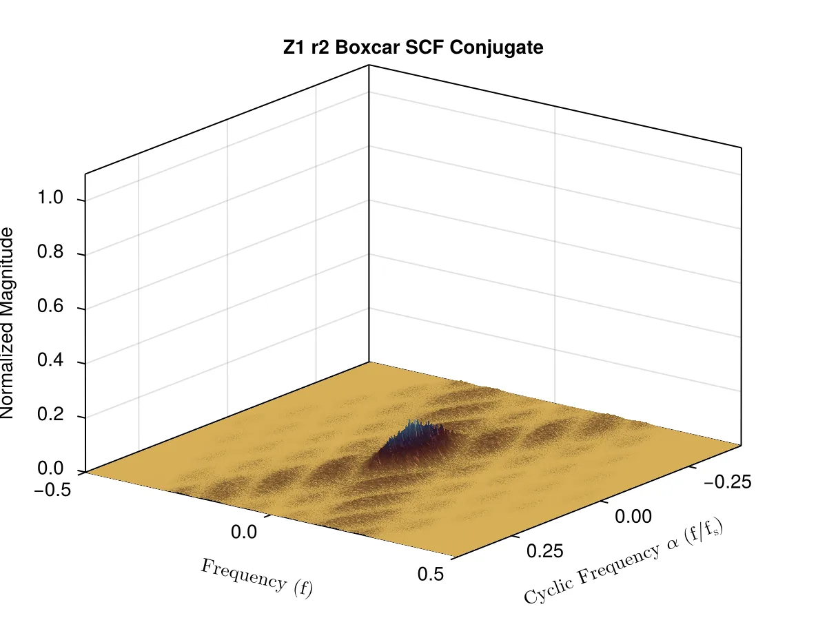
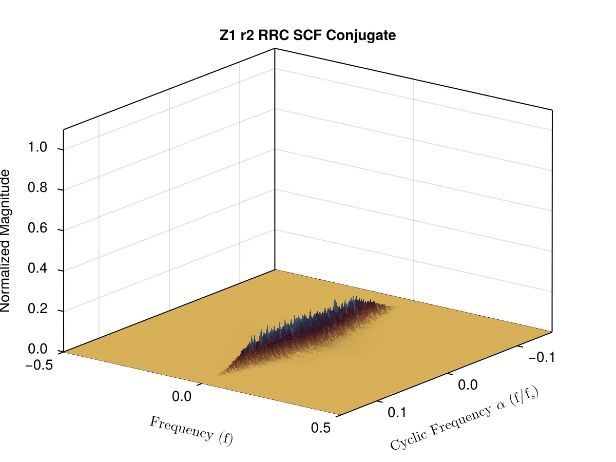
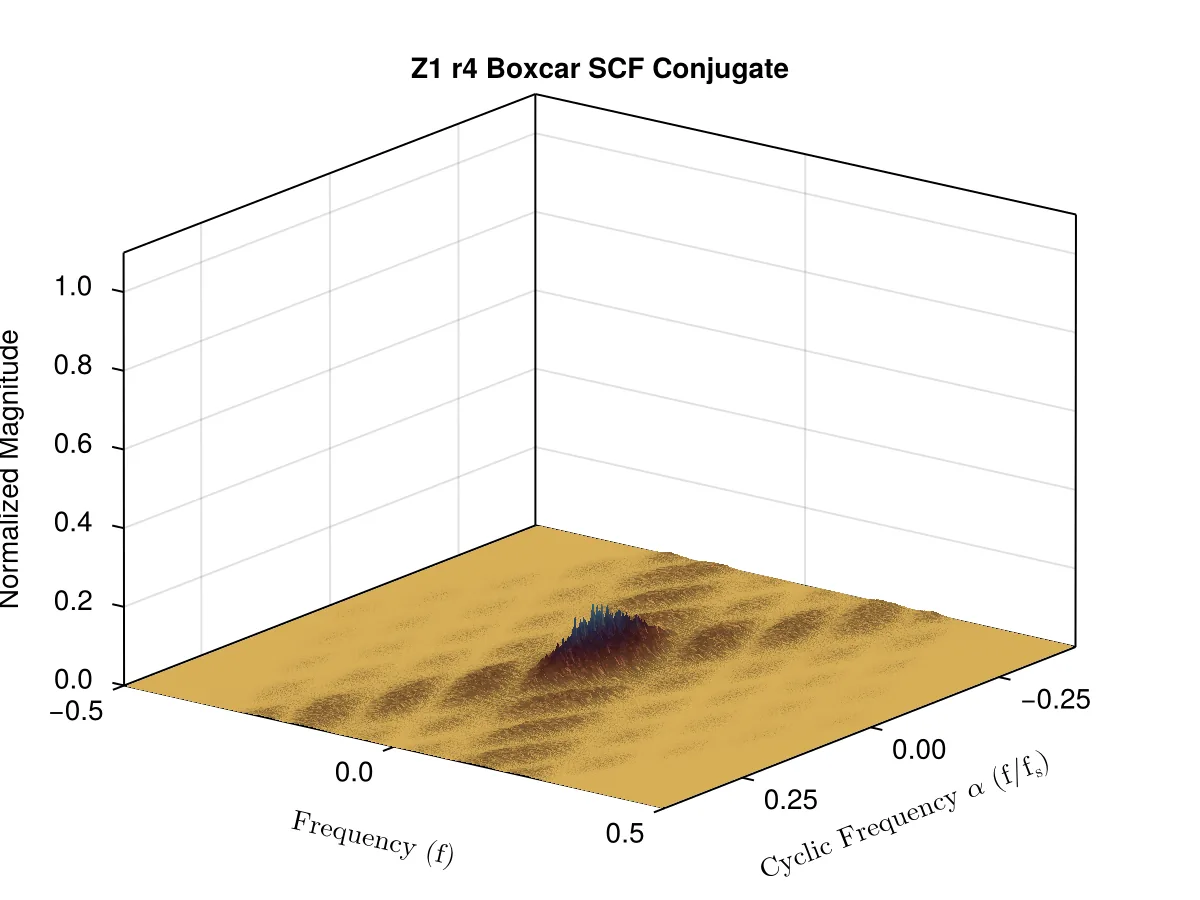
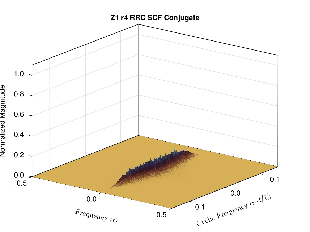
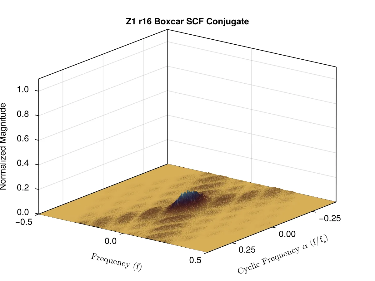
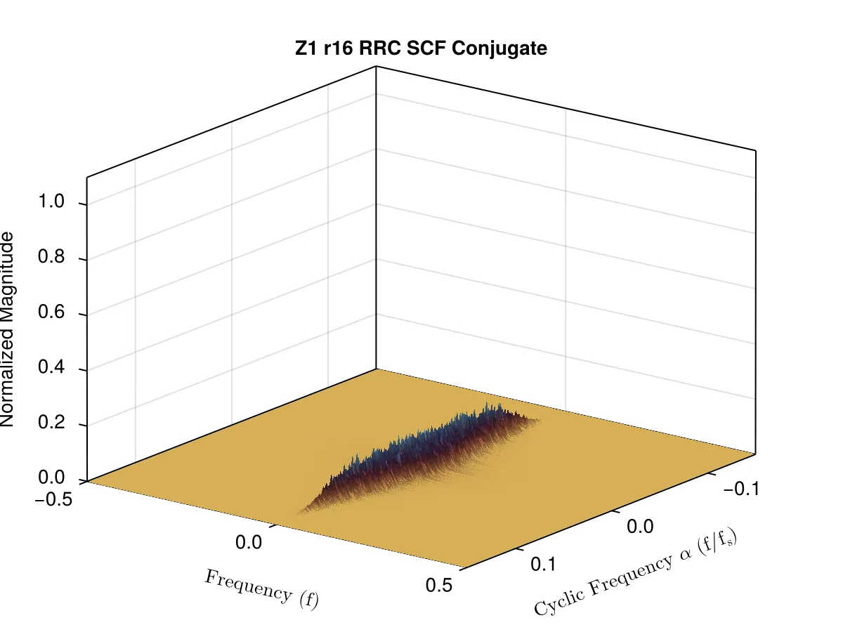
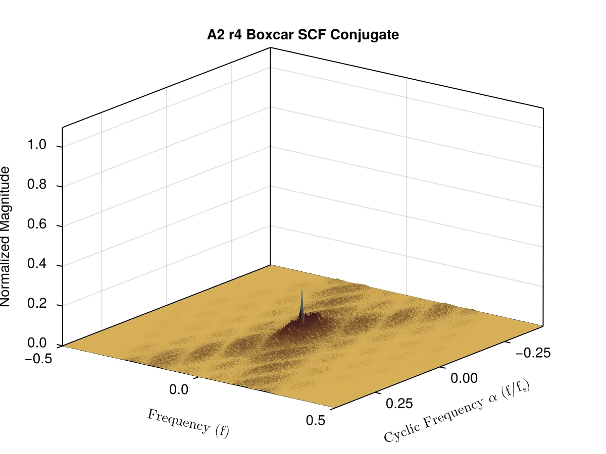
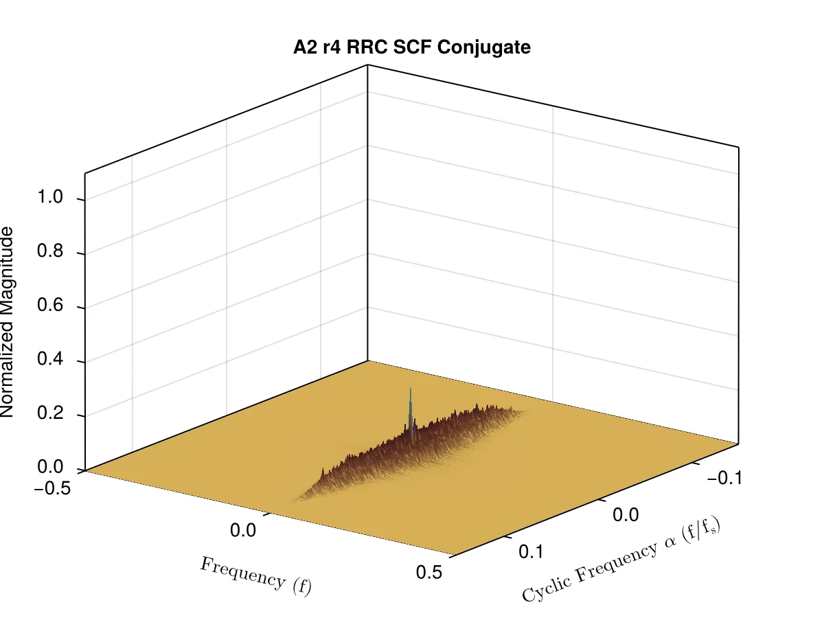
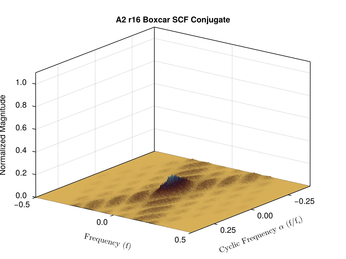
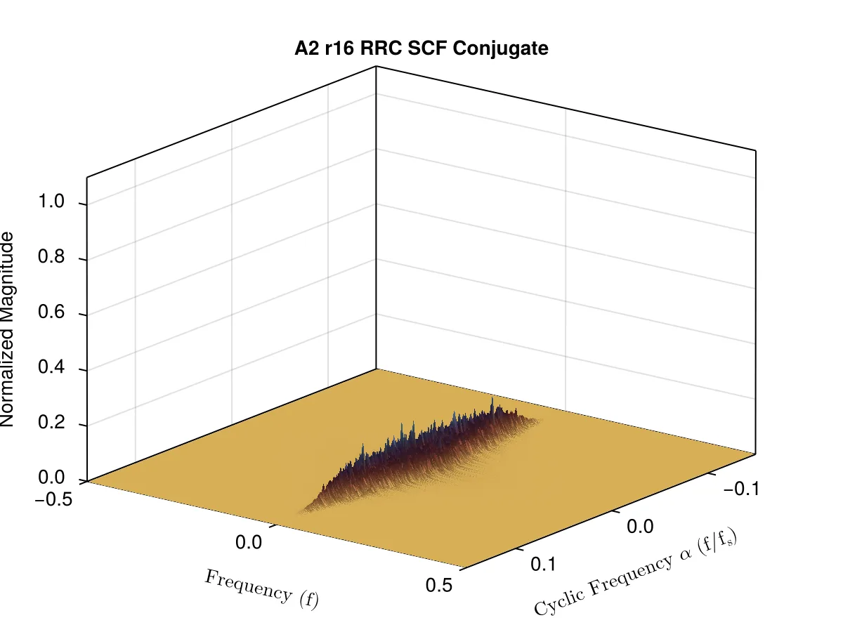
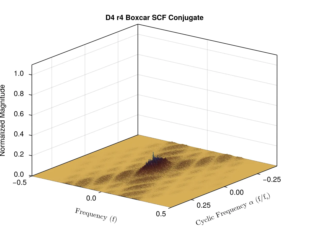
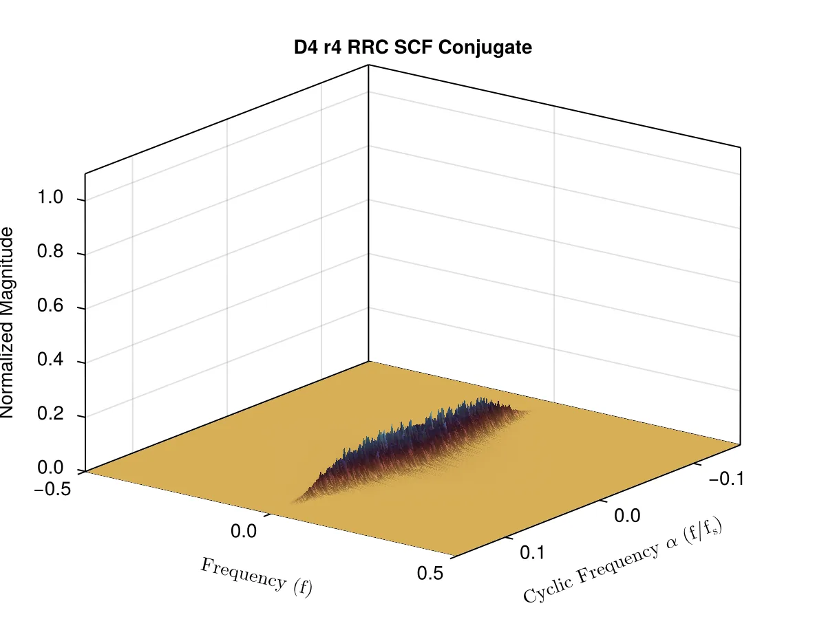
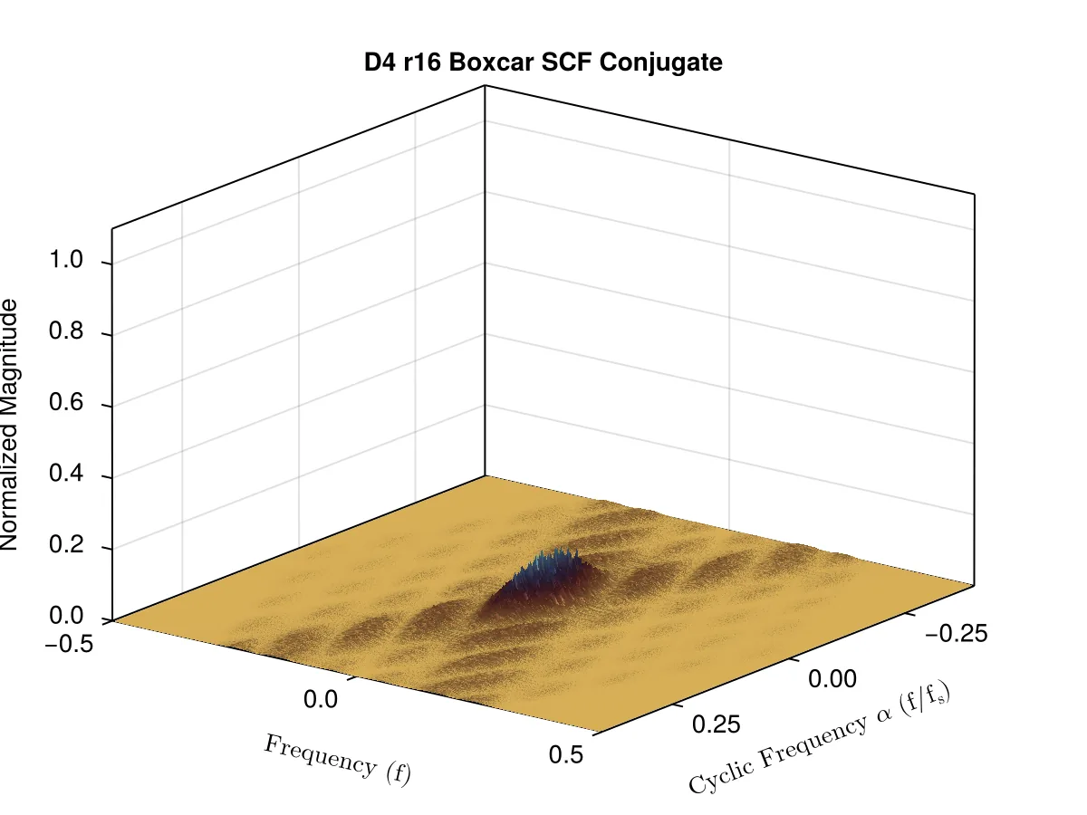
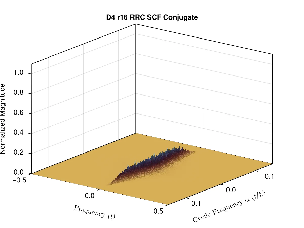
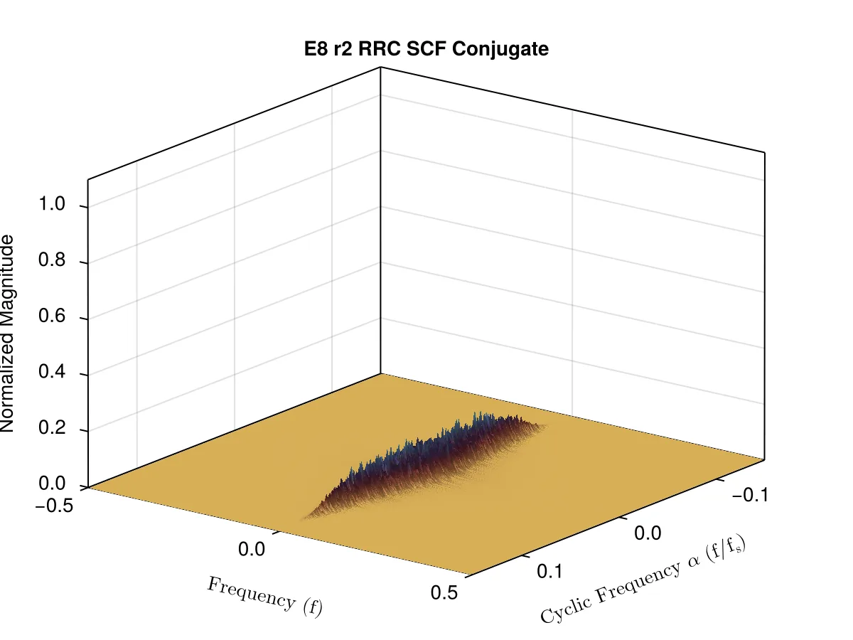
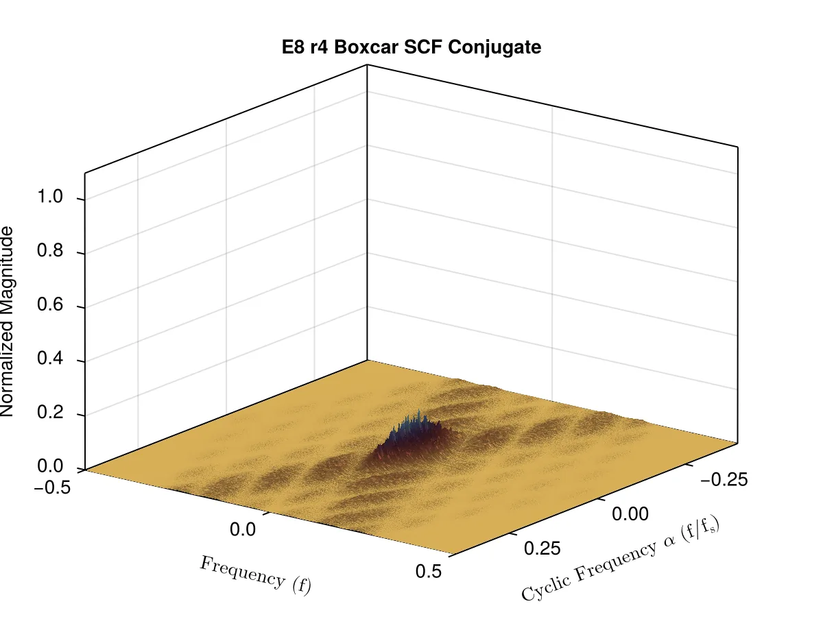
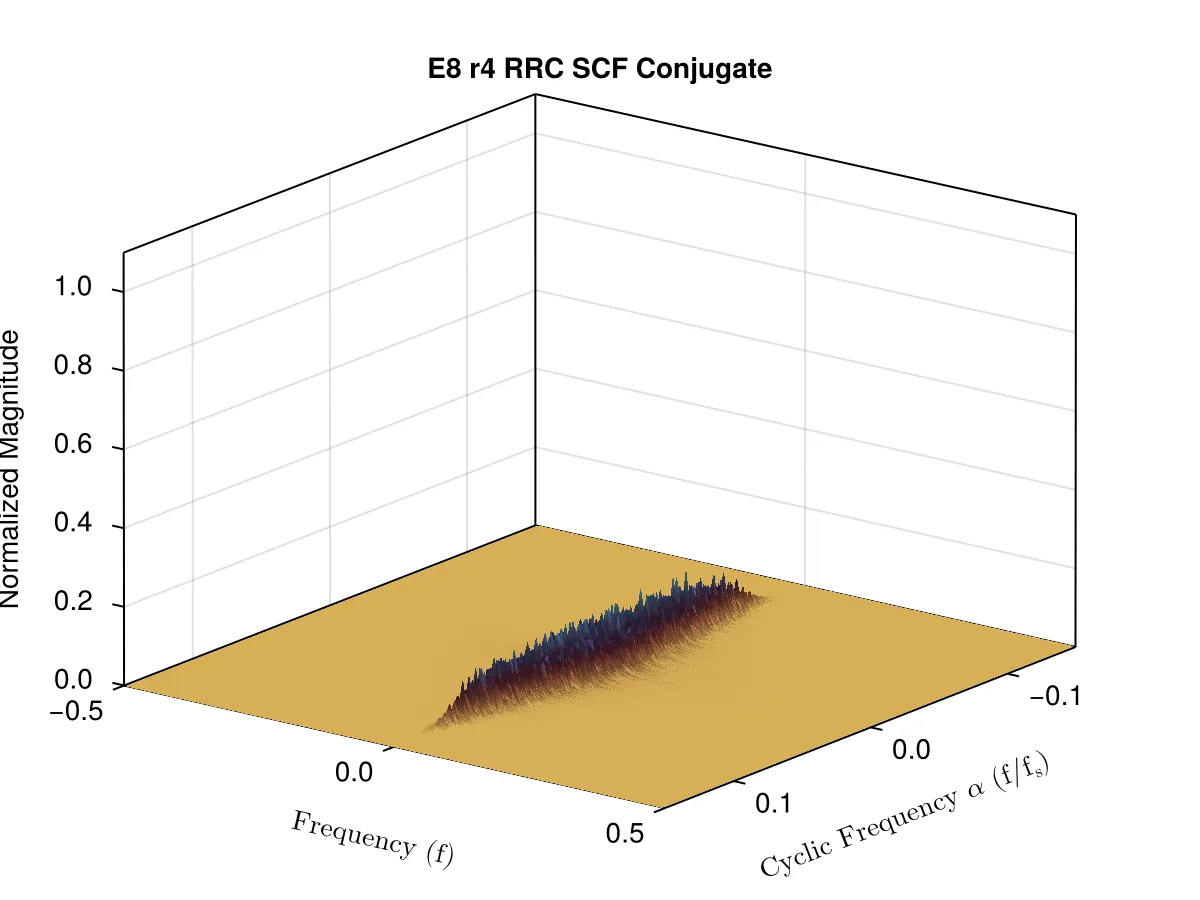
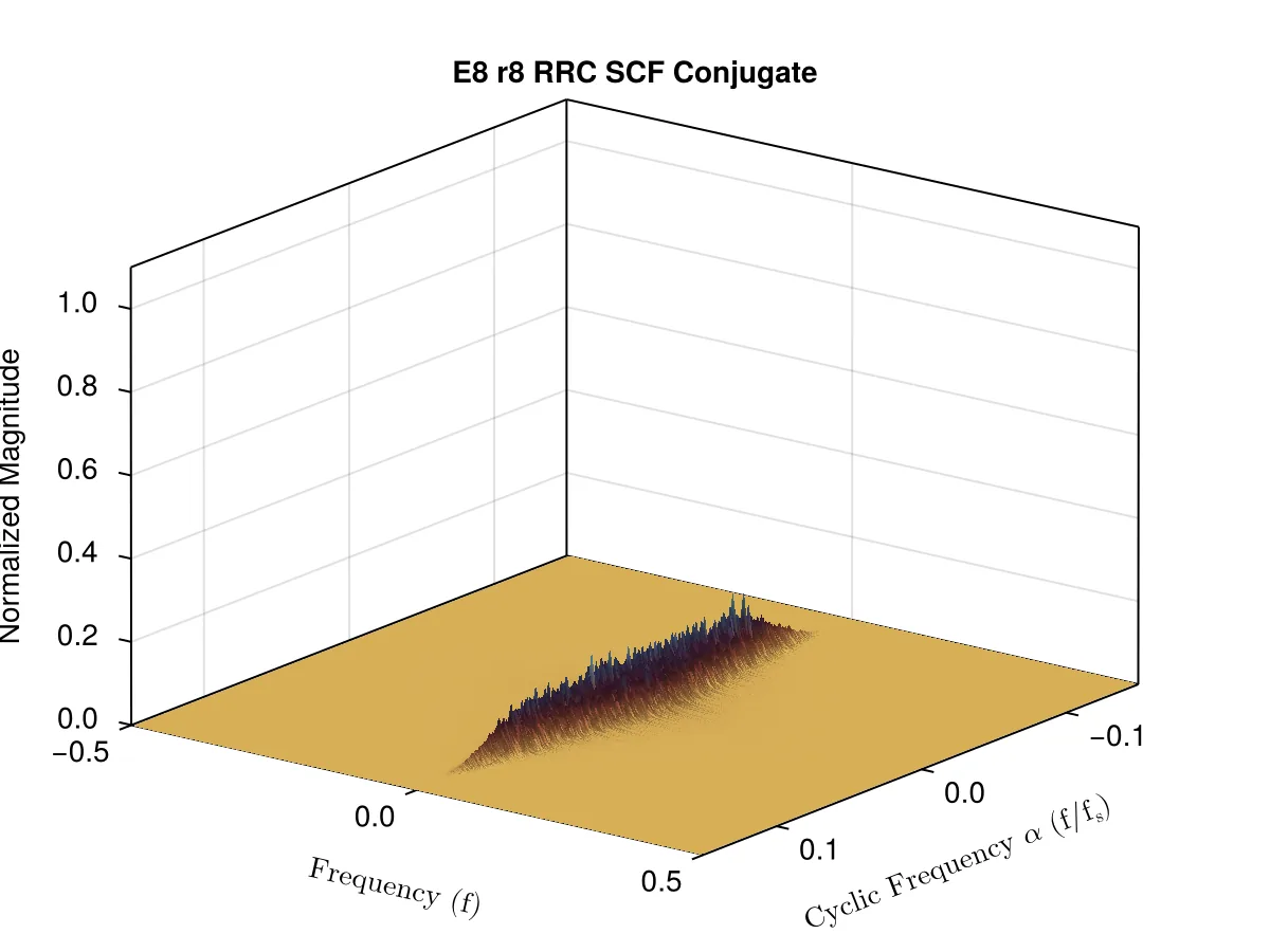
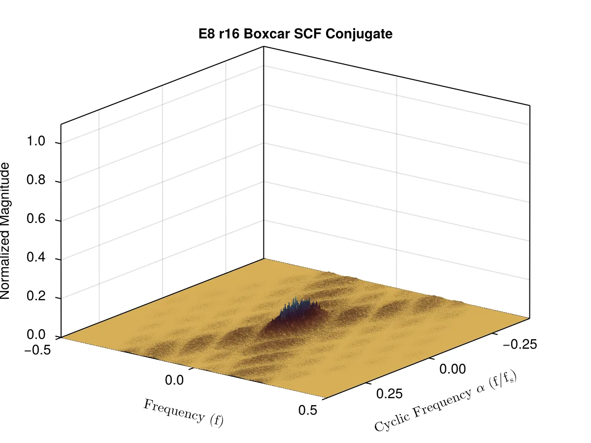
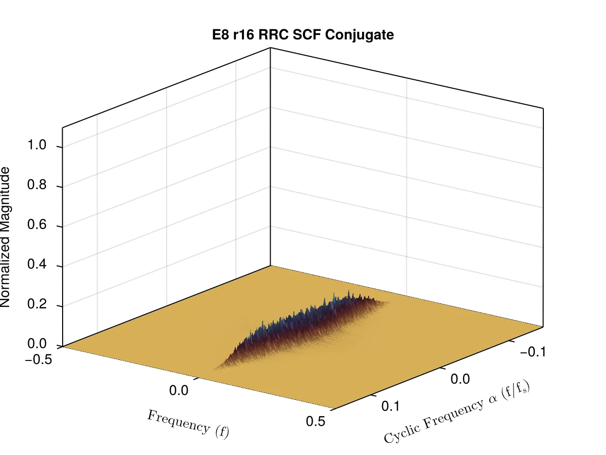
Similar to the CAF conjugate, the SCF conjugate highlights asymmetries in the constellation, but interprets the results in the frequency domain as opposed to the tau domain.

The CAF Conjugate and the SCF conjugate are “required to fully study the statistical structure of communication signals that have been … converted to complex baseband (zero frequency)” – Chad Spooner. While it is known that QAMs with more than 2 points in the constellation have only non-conjugate features, it is still important to fully characterize these lattice modulations with the conjugate versions of the CAF and SCF in order to confirm/deny that they also only contain non-conjugate features. More details on why we need conjugate versions at all can be found in Spooner’s work [10].

Citations

1. C. M. Spooner, “For the Beginner at CSP,” Cyclostationary Signal Processing, Jul. 14, 2019. [Online]. Available: https://cyclostationary.blog/2019/07/14/for-the-beginner-at-csp/
2. C. M. Spooner, “Conjugation Configurations,” Cyclostationary Signal Processing, Feb. 29, 2016. [Online]. Available: https://cyclostationary.blog/2016/02/29/conjugation-configurations/
3. A. Napolitano, Cyclostationary Processes and Time Series: Theory, Applications, and Generalizations. Academic Press, 2019.

Gallery

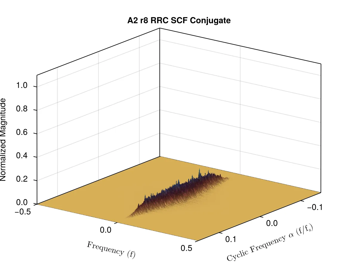
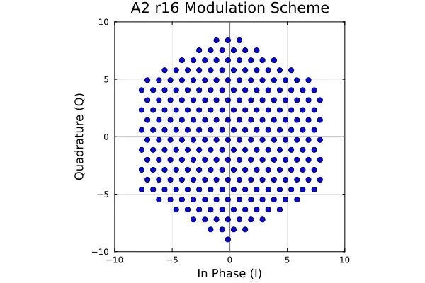
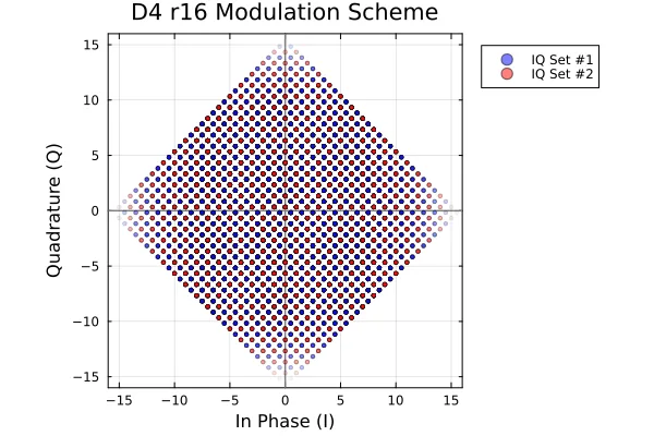
The following gallery shows the complete combination of CAF plots, alpha profiles, tau profiles, and CAF Conjugate plots at relevant alpha values of the Z1, A2, D4, and E8 lattice constellations with moduli ranging from r = 2, 4, 8, 16, grouped by type of pulse shaping filter as well as the equivalent QAM represented by the Z1(r) lattice. All data was analyzed at infinite SNR, so the “noise” floor shown is the correlation noise from non-correlated samples.

The gallery additionally shows the complete combination of SCF plots, alpha profiles, frequency-profiles, and SCF conjugate plots at relevant alpha values of the Z1, A2, D4, and E8 lattice constellations with moduli ranging from r = 2, 4, 8, 16, grouped by type of pulse shaping filter as well as the equivalent QAM represented by the Z1(r) lattice. All data was analyzed at infinite SNR, so the “noise” floor shown is the correlation noise from non-correlated samples.

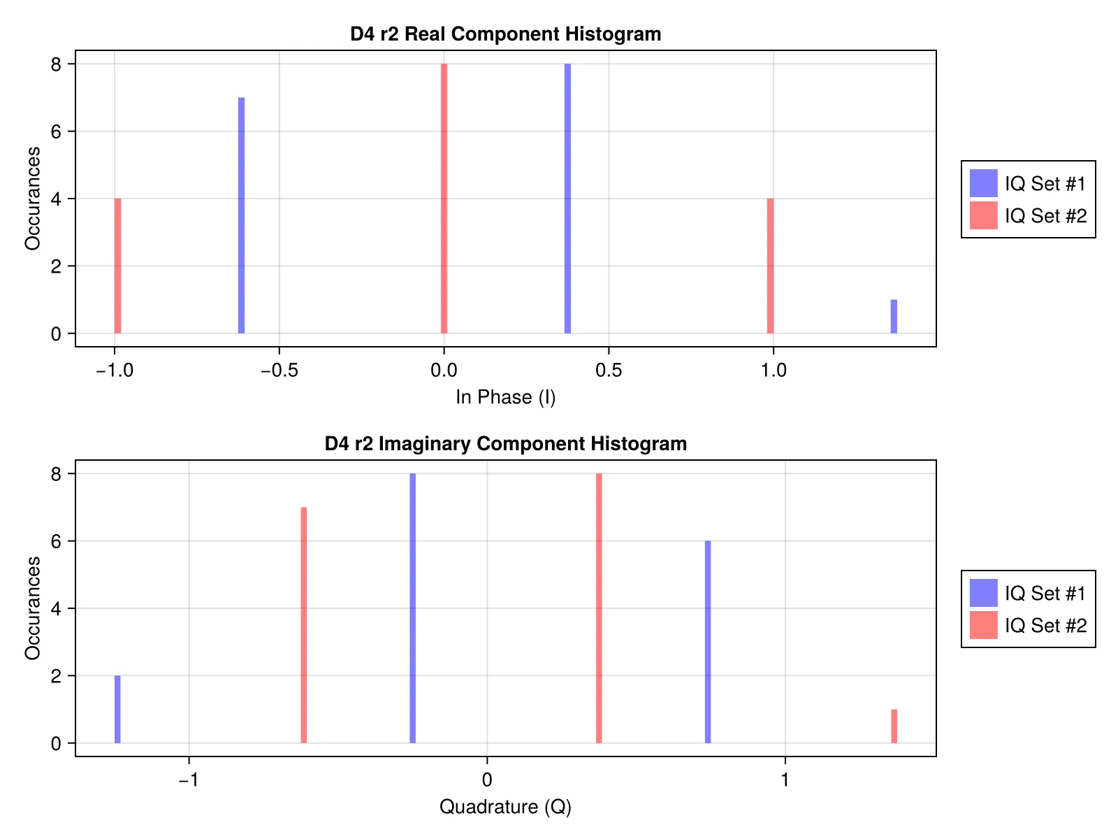
While most of the plots appear quite similar to the human eye, there is one notable distinction for the lattice D4 r2, which shows spikes in the alpha profile at multiples of the lattice symbol rate (1/20) in addition to multiples of the IQ symbol rate. These spikes disappear to the human eye for both higher moduli and the higher dimensional lattice E8.

Z1 Lattice

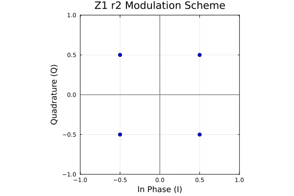
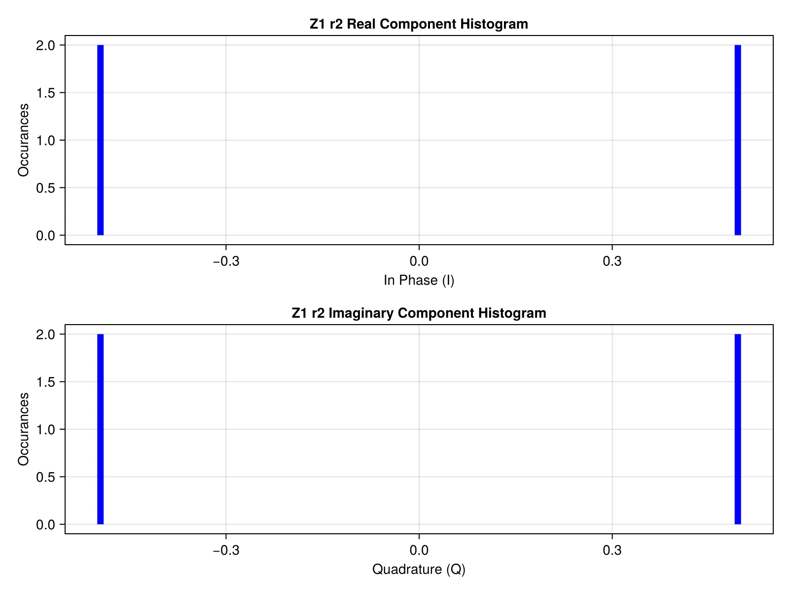
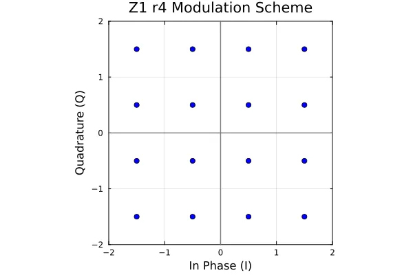
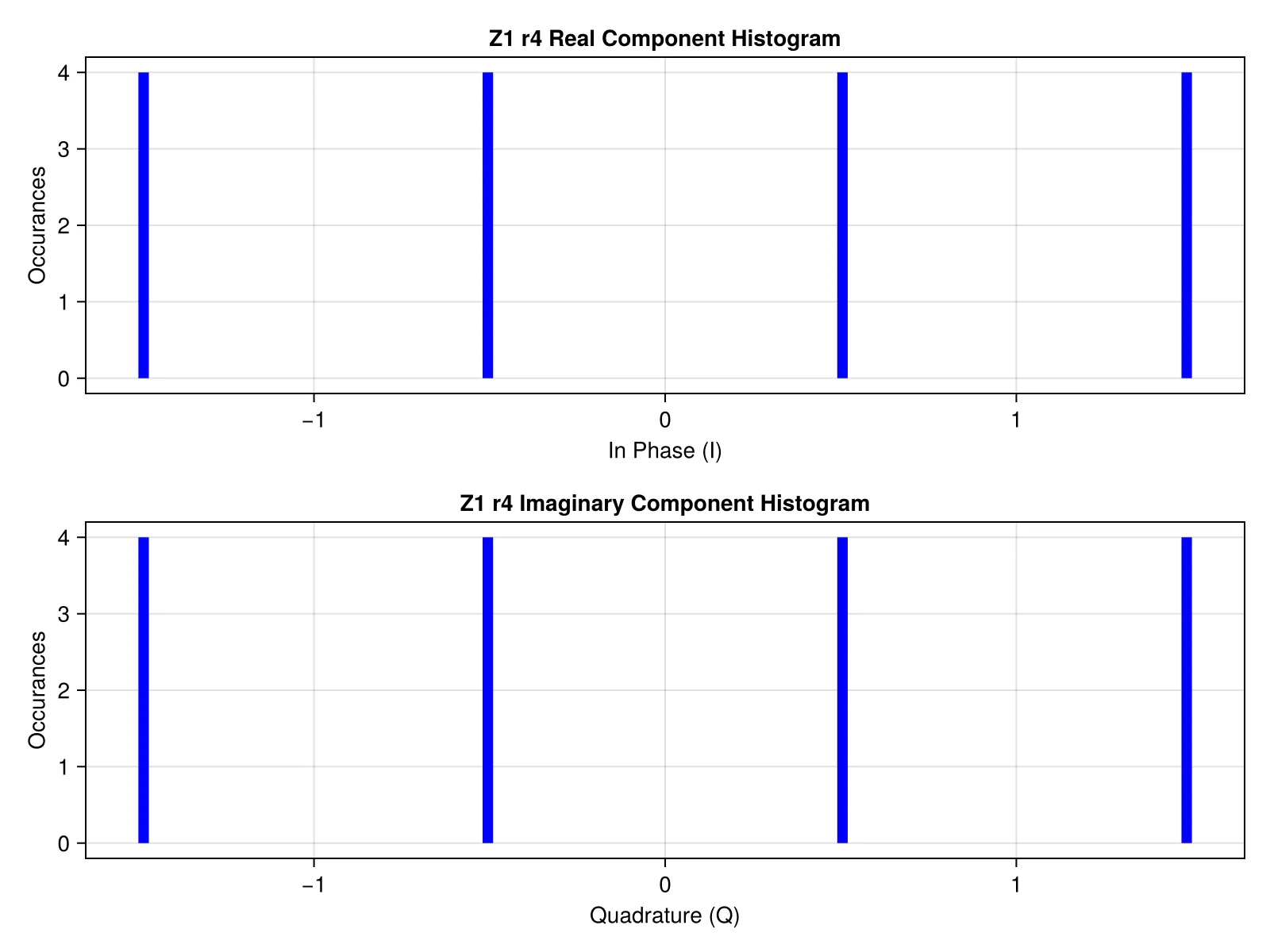
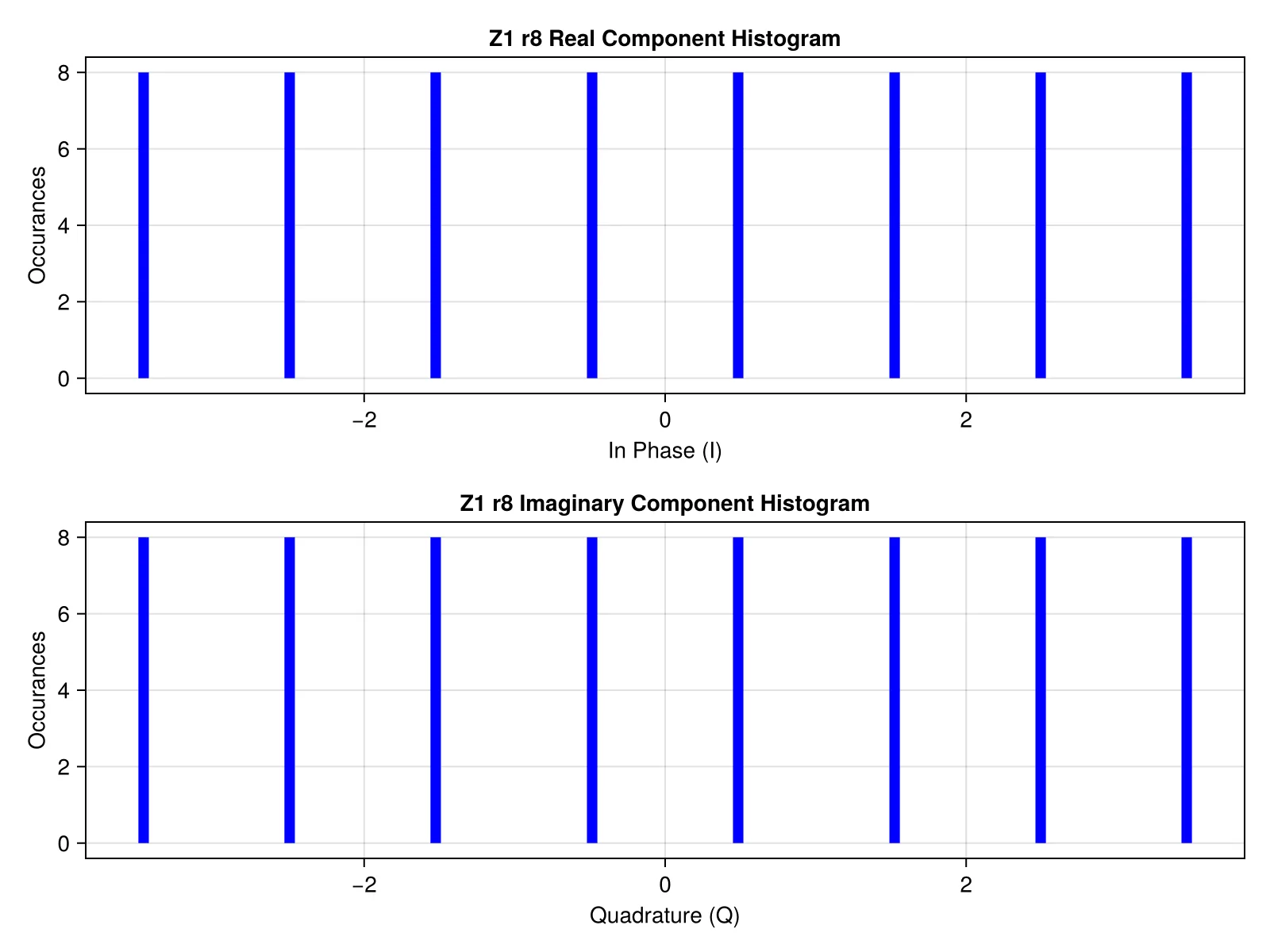
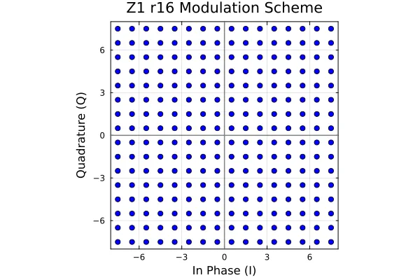
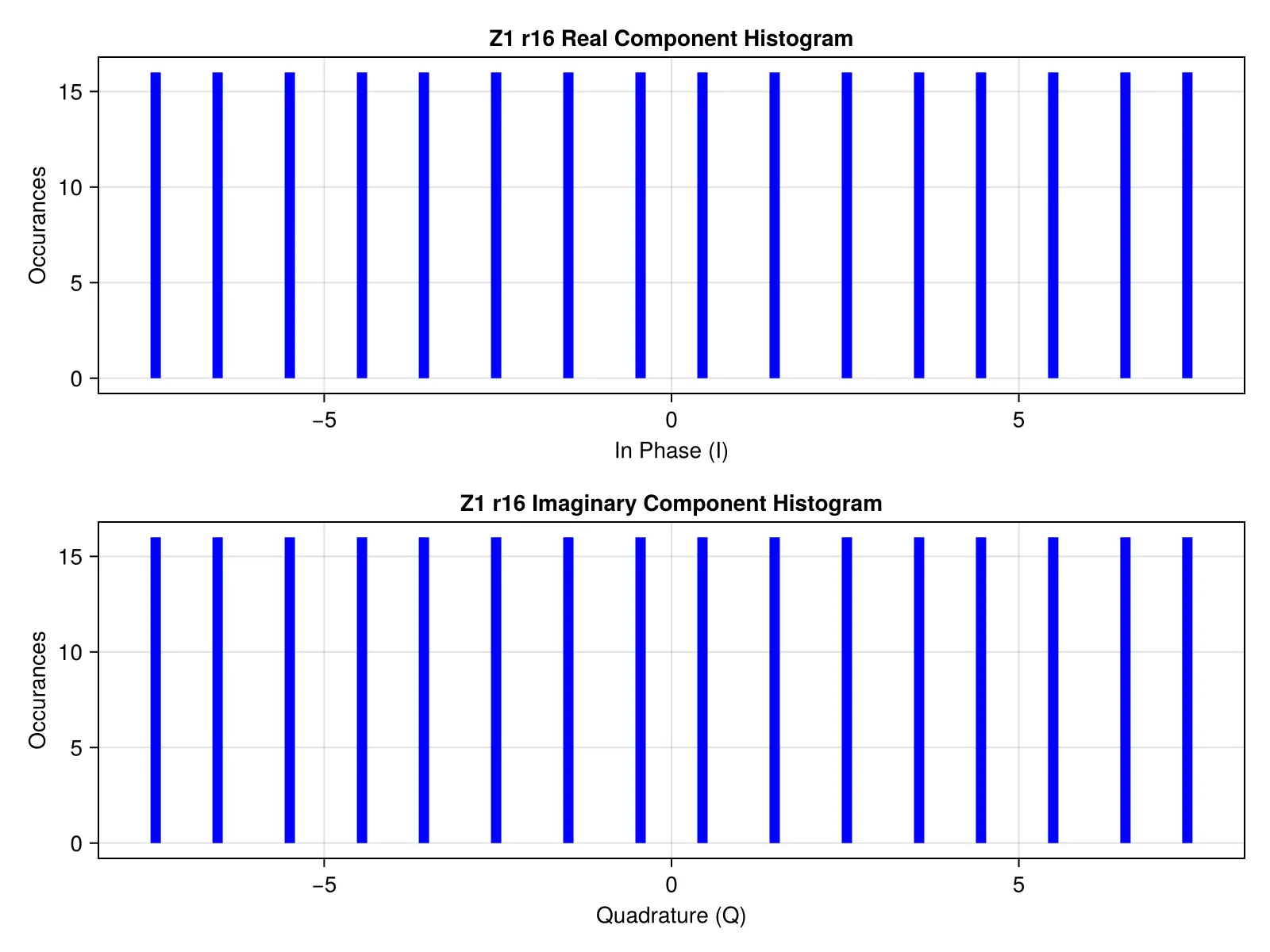
The Z1 lattice is equivalent to modern day modulation schemes like QPSK or QAMs. As opposed to denoting modulation order (:= the number of possible symbol states in the constellation) like typical QAMs, instead we denote the modulus (r) of the lattice. To convert between the two, use the following equation: modulation order = r². Below, we show IQ constellations for QAMs of various moduli, as well as their trivial histograms of the real and imaginary components separately. Motivation to look at each dimension independently in order to get a better sense of how the constellation is modulated into IQ symbols should become more evident for higher dimensional lattices, and is included here only for completeness.

QPSK Equivalent (Modulus r = 2)

Boxcar Filter

RRC Filter

16-QAM Equivalent (Modulus r = 4)

Boxcar Filter

RRC Filter

64-QAM Equivalent (Modulus r = 8)

Boxcar Filter

RRC Filter

256-QAM Equivalent (Modulus r = 16)

Boxcar Filter

RRC Filter

A2 Lattice

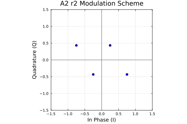
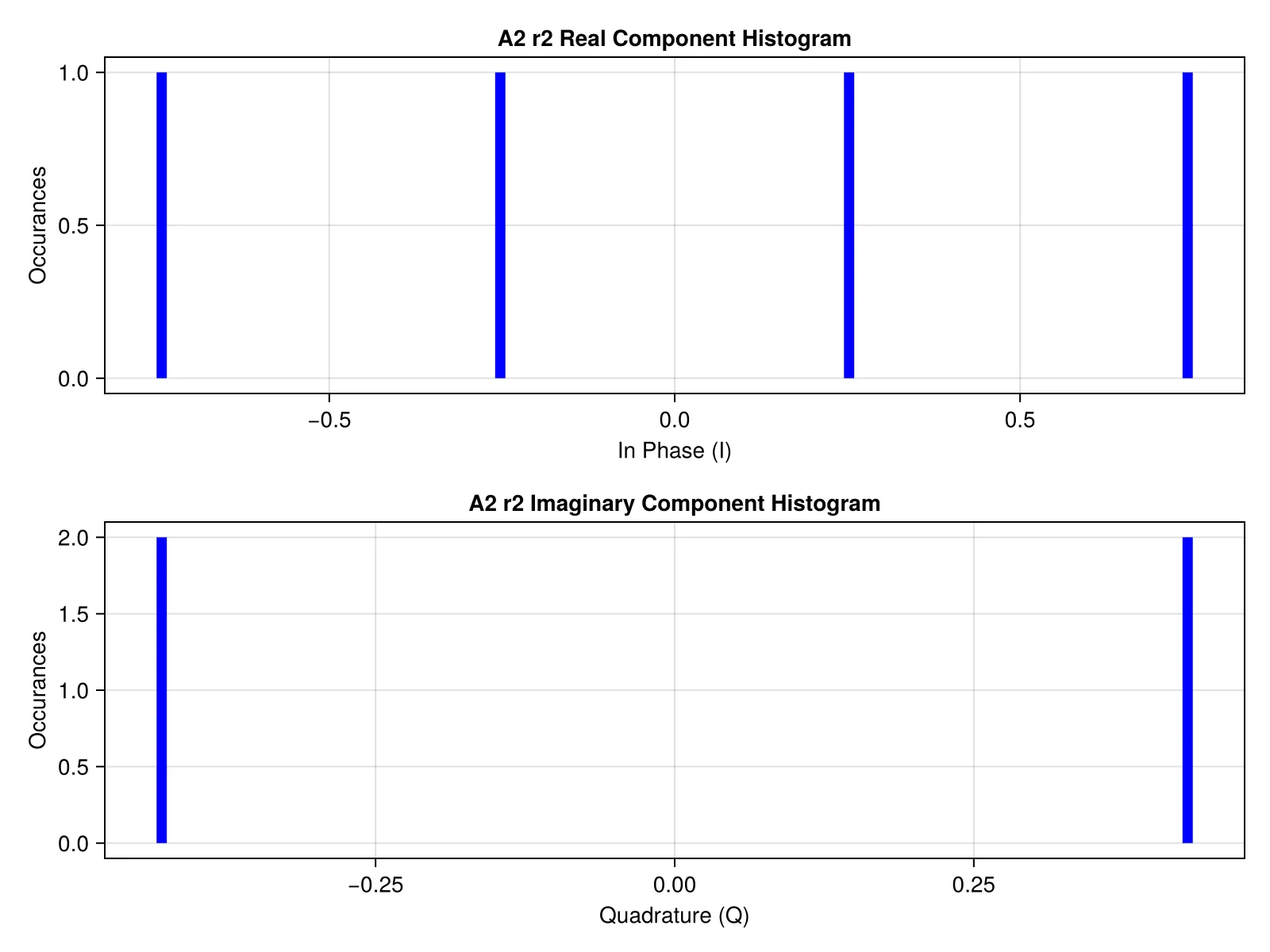
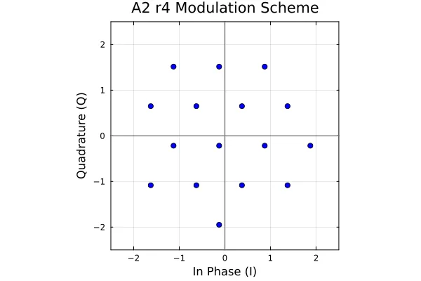
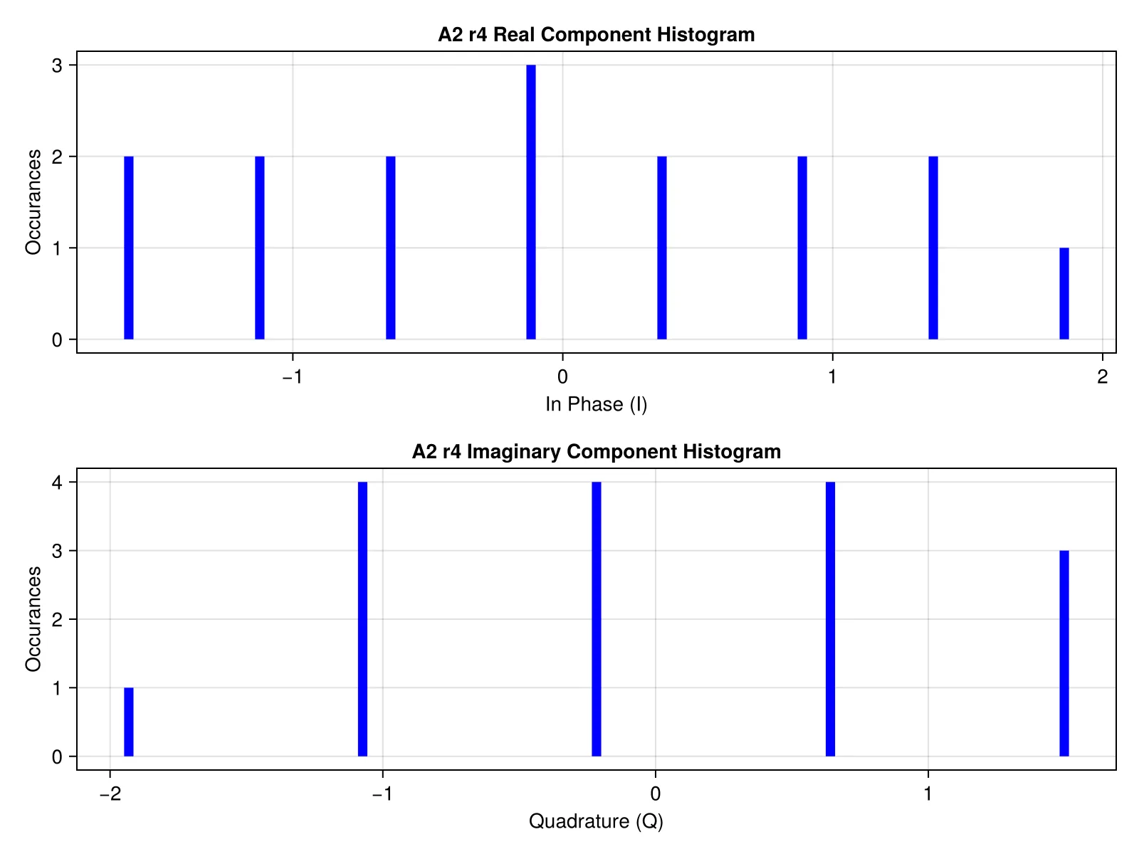
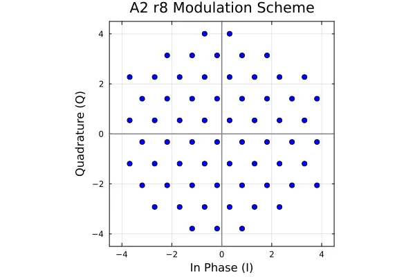
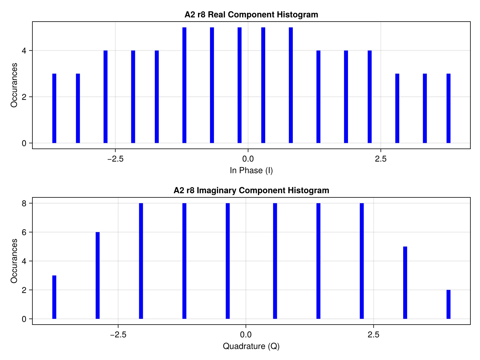
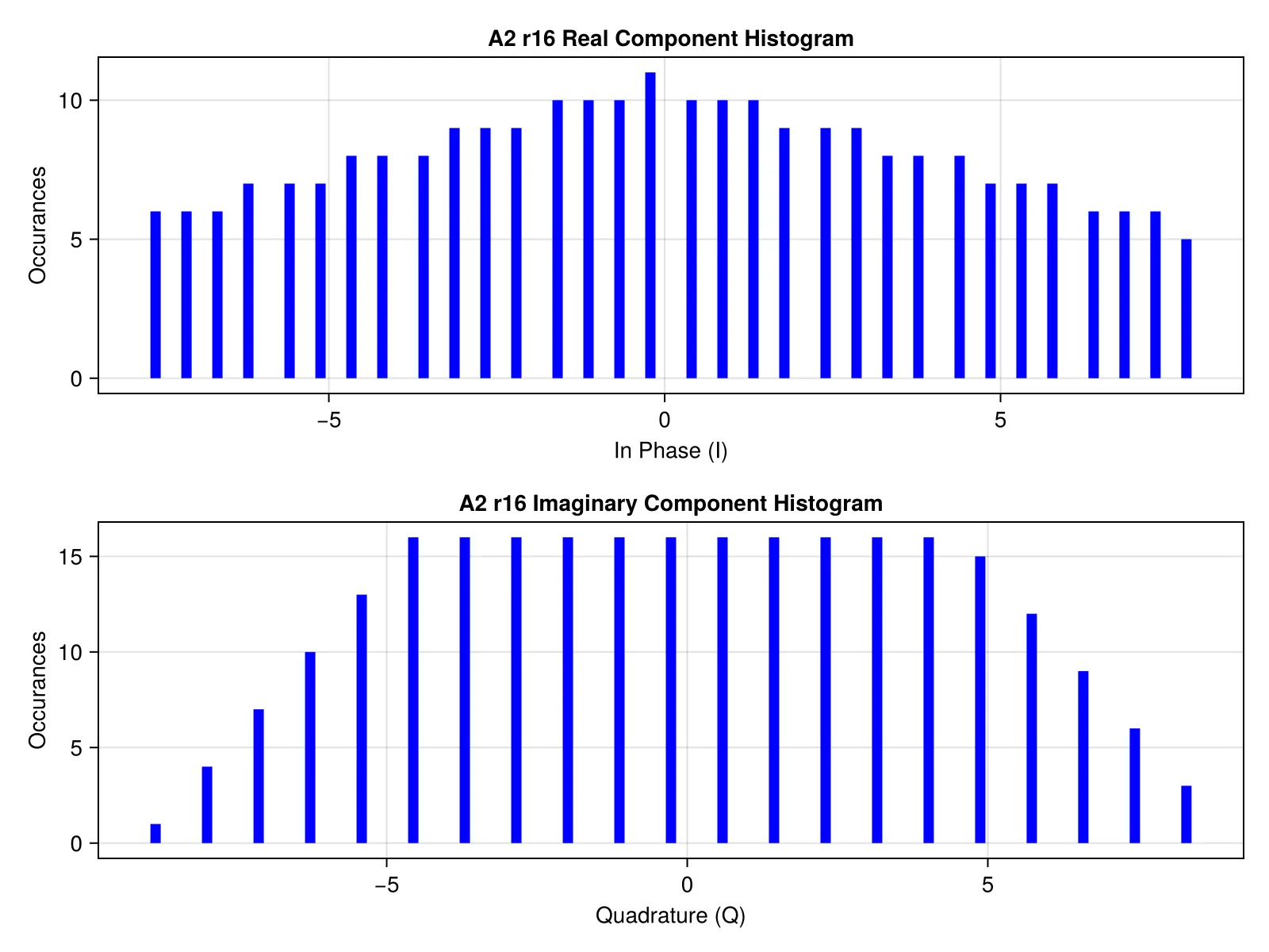
The first “interesting” lattice. It is still 2 dimensional, so each lattice point can trivially map to an IQ point. As r increases, the constellation will start to approximate a hexagonal region centered around the origin. Notice in the following A2 histograms, we see a trend as r increases, the lower power I and Q components are used more frequently than the higher power ones. This is a glimpse of how, even for the low, 2-dimensional A2 lattice, these lattices of interest have Voronoi cells that are better approximations of n-dimensional spheres than the rectangular QAMs.

QPSK Comparable (Modulus r = 2)

Boxcar Filter

RRC Filter

16-QAM Comparable (Modulus r = 4)

Boxcar Filter

RRC Filter

64-QAM Comparable (Modulus r = 8)

Boxcar Filter

RRC Filter

256-QAM Equivalent (Modulus r = 16)

Boxcar Filter

RRC Filter

D4 Lattice

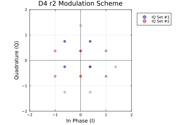
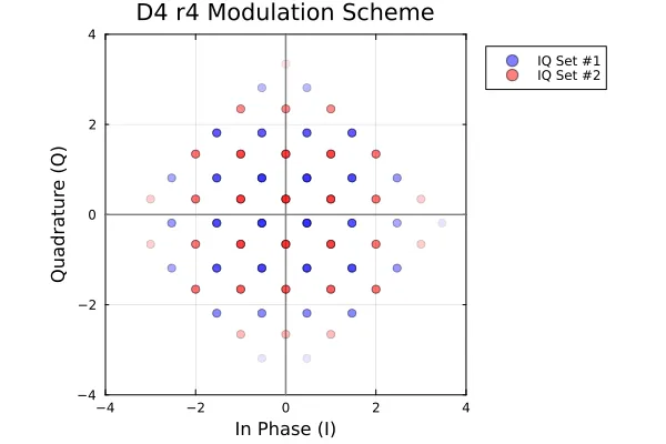
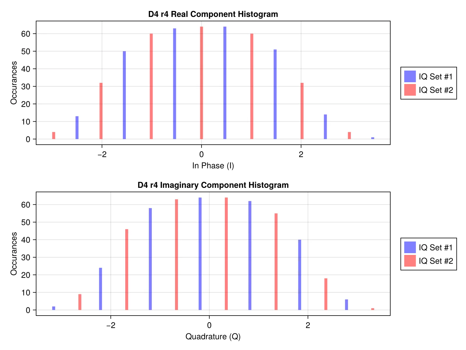
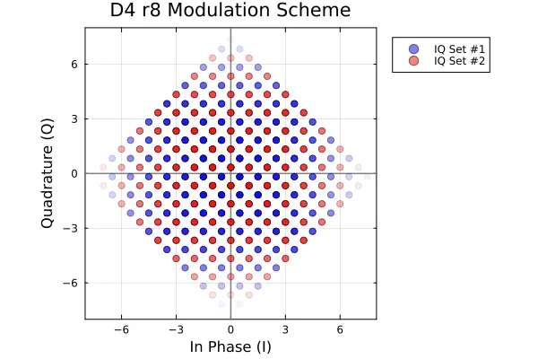
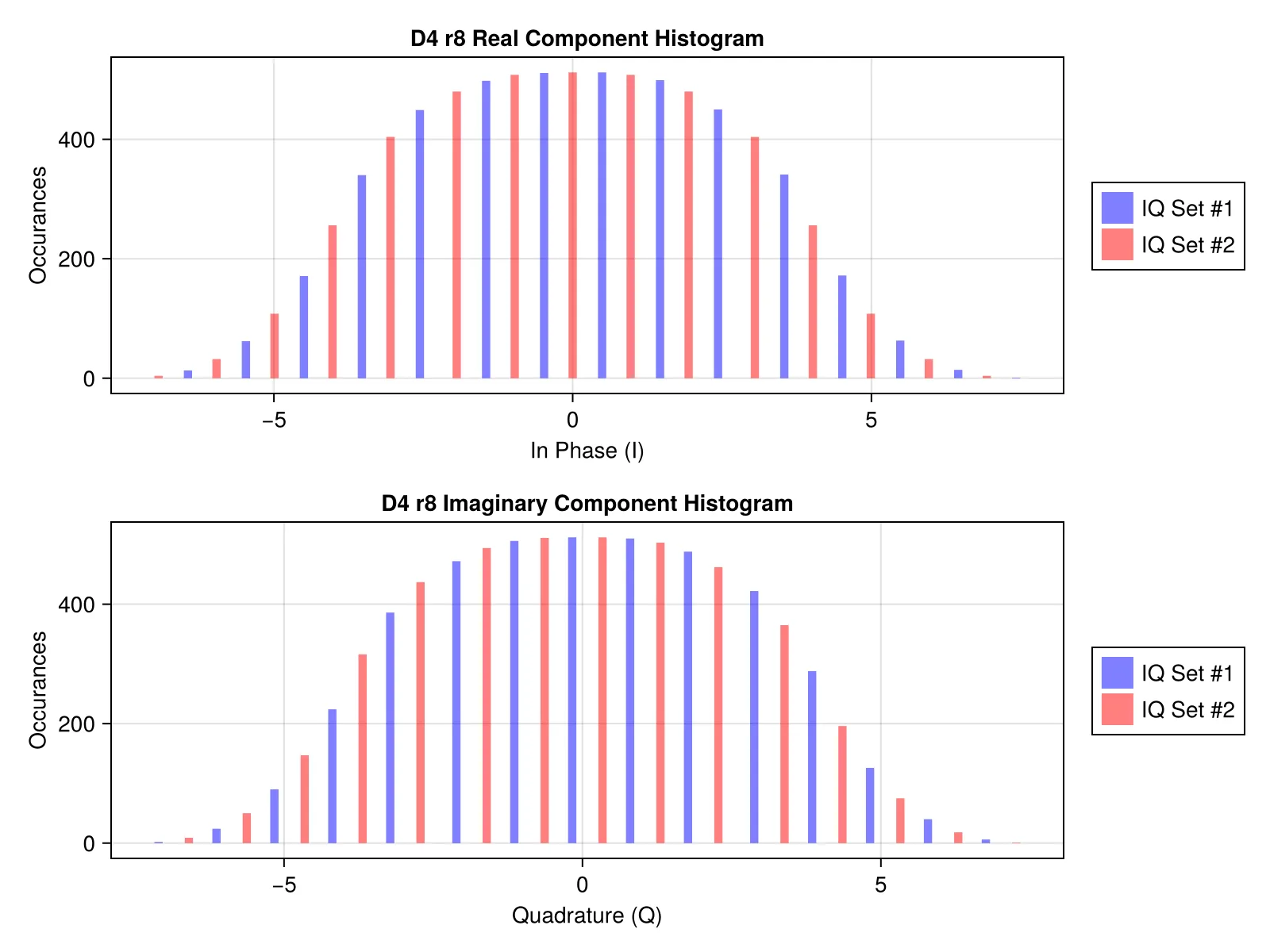
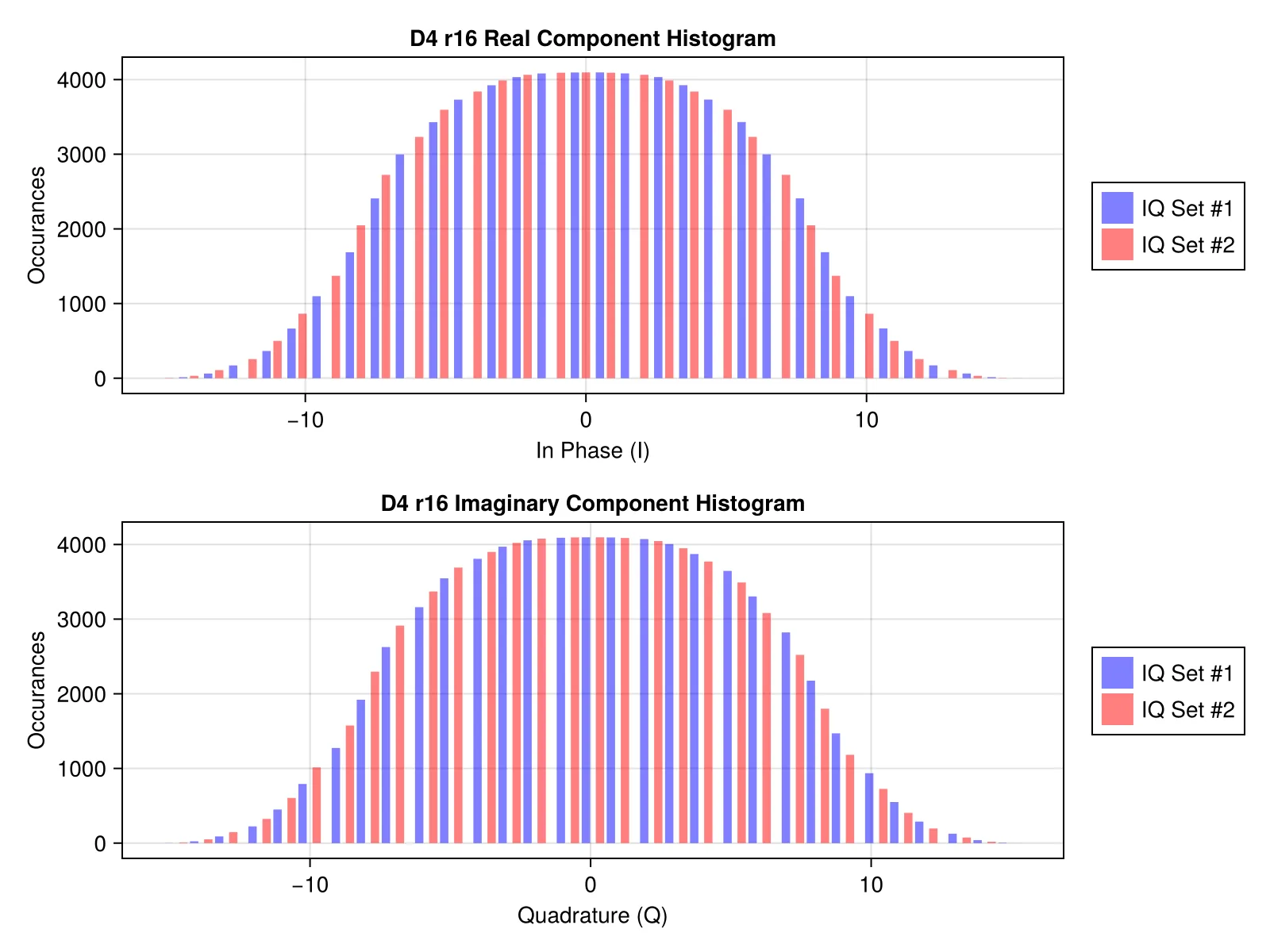
Now we discuss the first lattice presented with more than 2 dimensions: D4. In order to modulate into 2-dimensional IQ points, we simply split each 4-dimensional lattice point into 2 IQ points. Each set of IQ points is differentiated using different colors in the plots below. The transparency of each point has been adjusted so that overlapping points are darker, giving some semblance of probability occurrences. As we saw with A2, the histograms appear more and more gaussian as r increases, again revealing how the D4 Voronoi cell approximates the 4-sphere.

QPSK Comparable (Modulus r = 2)

Boxcar Filter

RRC Filter

16-QAM Comparable (Modulus r = 4)

Boxcar Filter

RRC Filter

64-QAM Comparable (Modulus r = 8)

Boxcar Filter

RRC Filter

256-QAM Comparable (Modulus r = 16)

Boxcar Filter

RRC Filter

E8 Lattice

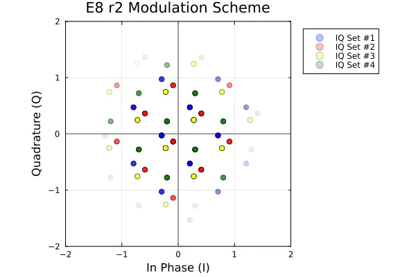
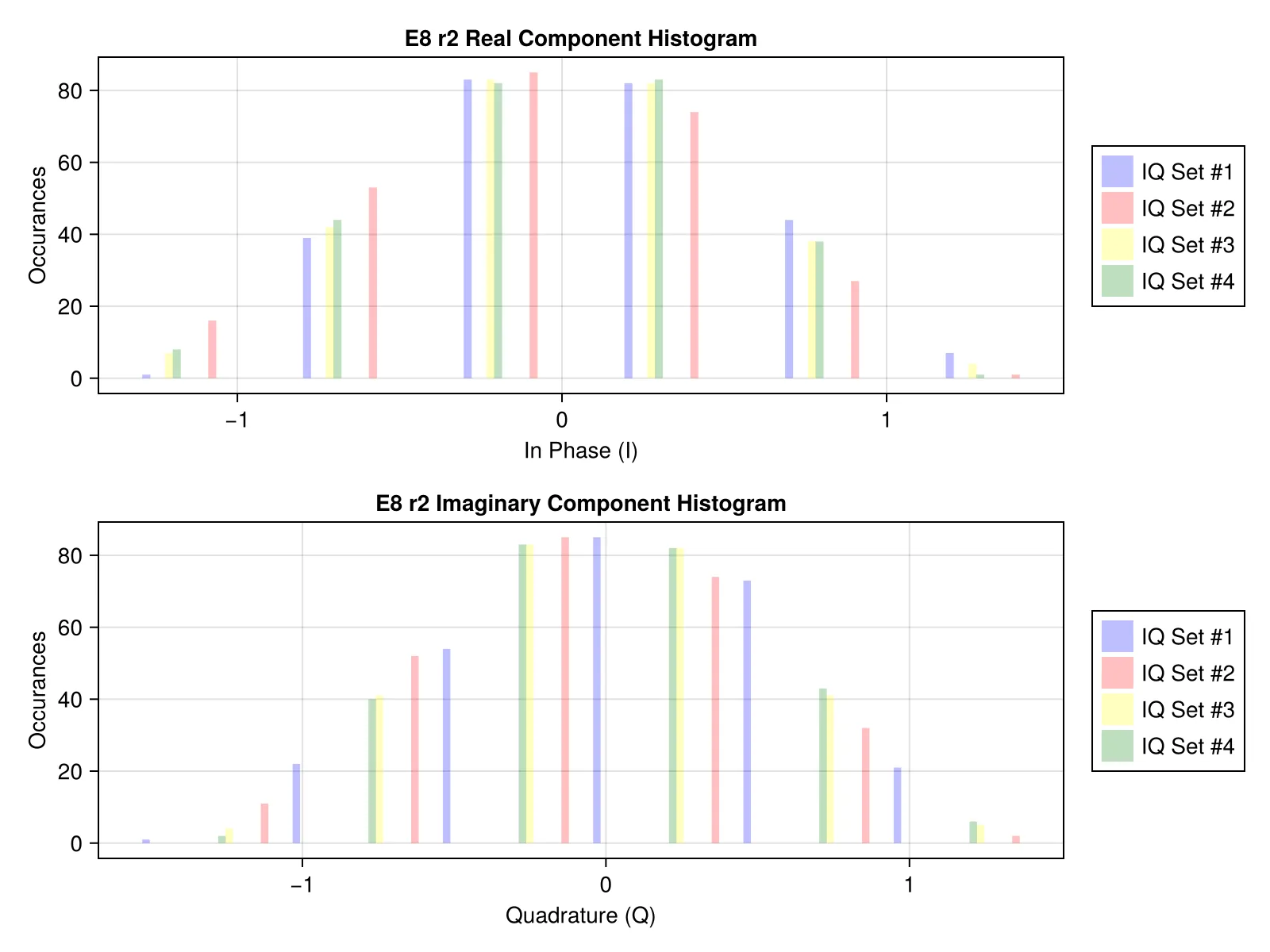
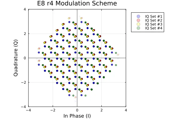
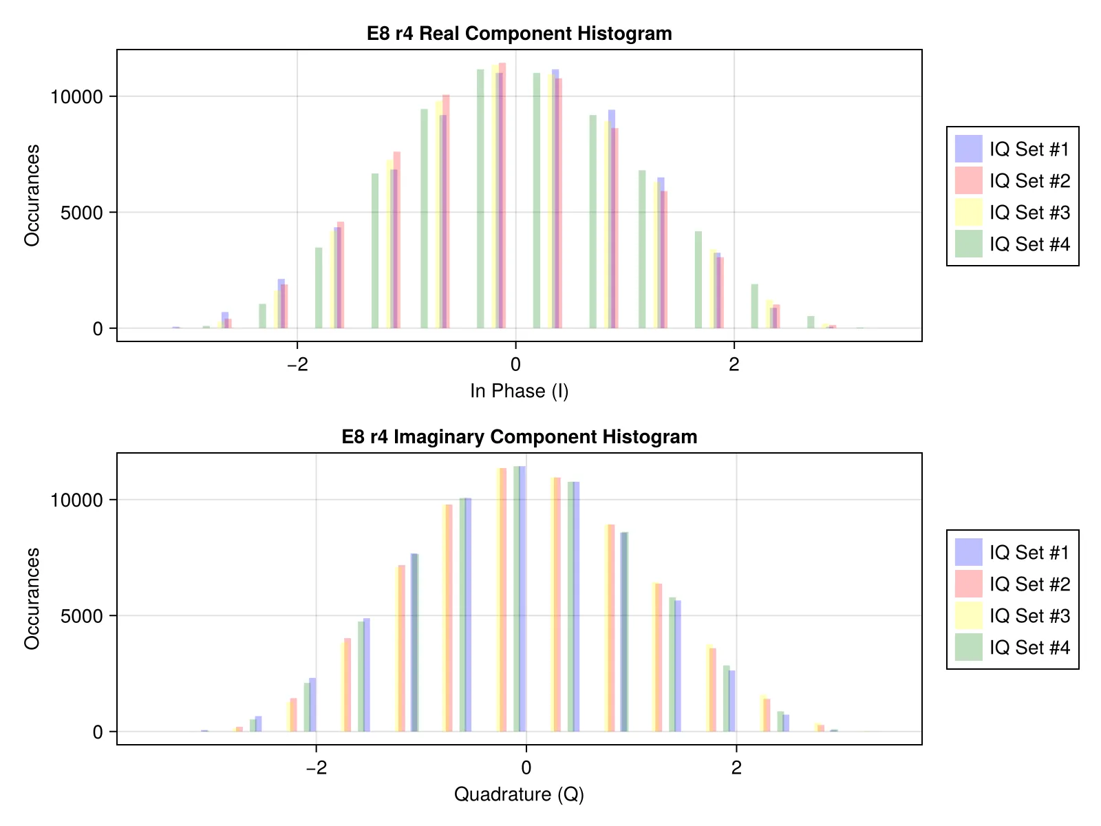
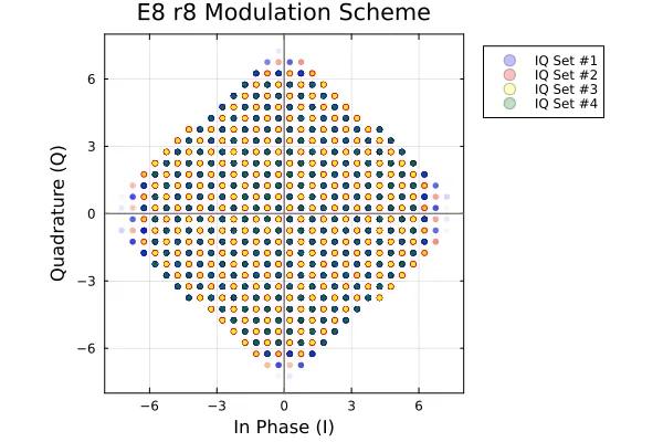
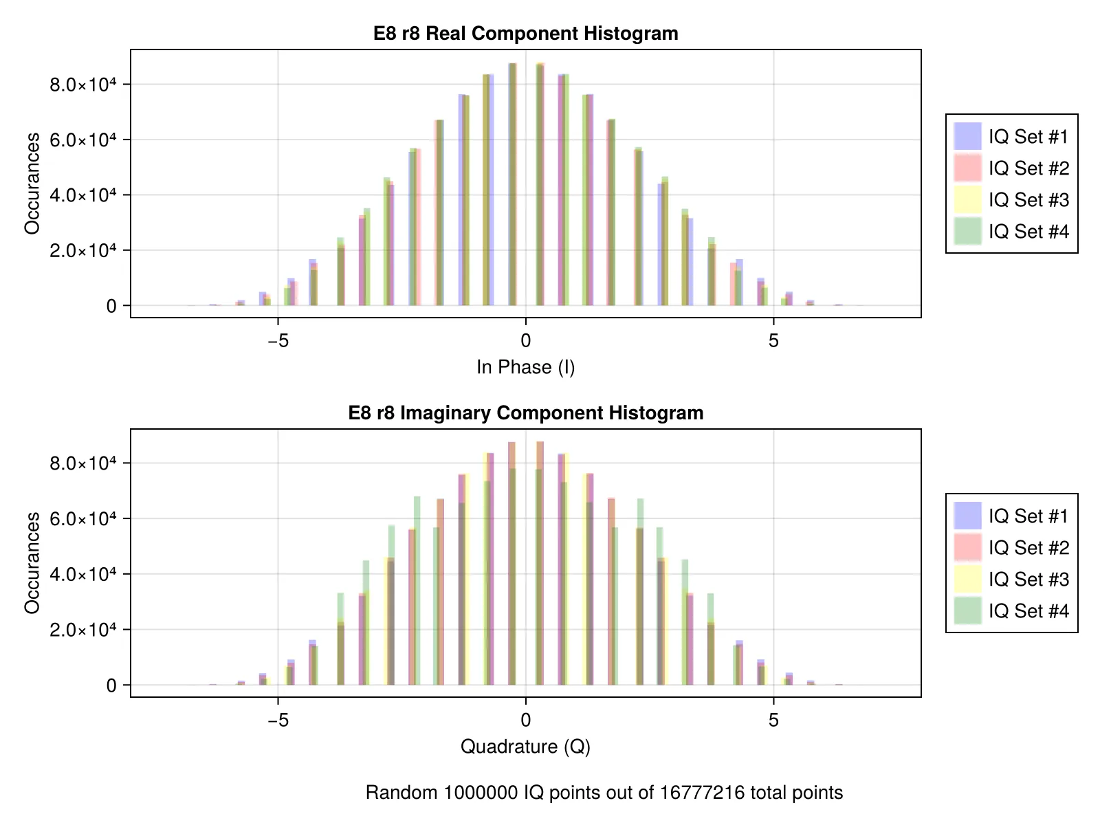
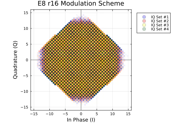
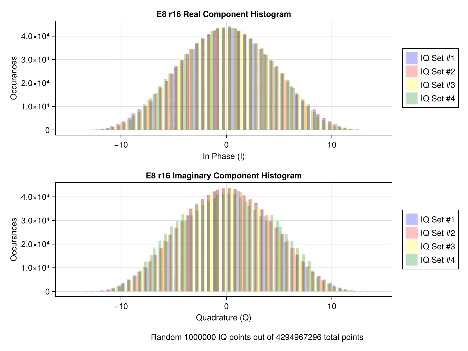
Similar to how a 4-dimensional D4 lattice point is split among 2 IQ points, an 8-dimensional E8 lattice point is split into 4 IQ points. Each set of IQ points is differentiated using different colors in the plots below. Due to the increasingly large number of possible constellation points for high modulus E8 lattices (scaling with n^r), the number of lattice points plotted is capped at 1 million. The transparency of each point has been adjusted so that overlapping points are darker, giving some semblance of probability occurrences. As we saw with A2 and D4, the histograms appear more gaussian-like as r increases, showing a glimpse of how E8’s Voronoi approximates the 8-sphere. Out of all of the lattices tested here, E8’s Voronoi cell is the best approximation of its own respective n-sphere.

QPSK Comparable (Modulus r = 2)

Boxcar Filter

RRC Filter

16-QAM Comparable (Modulus r = 4)

Boxcar Filter

RRC Filter

64-QAM Comparable (Modulus r = 8)

Boxcar Filter

RRC Filter

256-QAM Comparable (Modulus r = 16)

Boxcar Filter

RRC Filter

Discussion

As a general note, outside of a few specific cases of D4 r2 and some of the low modulus CAF Conjugate and SCF Conjugate plots (which are talked about more below), there is little to no variation to the human eye between most of the CAF, CAF Conjugate, SCF, and SCF Conjugate plots when compared with the same pulse shaping filter. This was expected for Z1, since it is known that higher order QAM modulations require higher order cyclic cumulants to differentiate them. This was previously unknown (to us, at least) for general lattices, but we believe our results confirm that any further analysis would likely require higher order cyclic cumulants.

CAF Features at Modulus r = 2

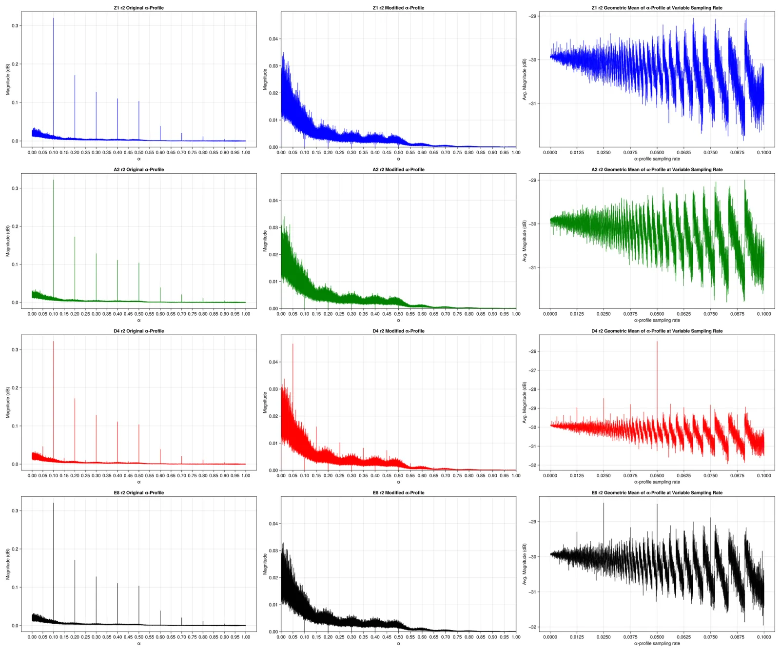
It has been acknowledged that there is a notable distinction for the lattice D4 r2 alpha profiles. While the human eye may struggle to detect any differences between the Z1, A2, and E8 r2 alpha profiles, that does not mean that there are no analyses that highlight any differences. One such example that highlights the D4 and E8 lattice symbol rates (1/20 and 1/40, respectively) is shown below.

This analysis relies on taking the geometric means of specific subsets of the alpha profiles, where each subset corresponds to skipping every n elements in the alpha profile. For example, subset 1 averages every 1 sample and is the geometric mean of the entire alpha profile. Subset 2 averages every other sample, subset 3 averages every 3 samples, etc. Note that since there are 81,920 elements of these alpha profiles, subset 8192 corresponds to alpha = 0.1 and averages only 10 samples. Also note that since 4096 * 2 = 8192, subset 4096 (alpha = 0.05) includes every element of subset 8192, as does every subset that is a power of 2. Therefore, if there exists a recurring spike at alpha values of 0.1, we should also expect spikes at 0.1 / 2 = 0.05, 0.1 / 4 = 0.025, 0.1 / 8 = 0.0125, etc.

One issue is that the known spikes in the alpha profile at multiples of 0.1 are significantly higher in magnitude compared to the rest of the alpha profile and will drown out any differences in the lattice modulations, even for D4 r2 that has the most visible spikes at multiples of 0.05. In order to remove this influence, a modified alpha profile is created by setting all of the alpha profile elements at multiples of 1/10 to identically 0. This modified alpha profile is shown in column 2 below.

The results from running the describe analysis on these modified alpha profiles is shown in column 3 below. The y-axis represents the geometric mean in dB of the alpha profile elements, and the x-axis corresponds to the alpha value of the first element of the alpha subset to be averaged.

Z1 and A2 do not show any significant spikes, indicating that the only significant spikes in their alpha profiles correspond to multiples of 0.1.

D4 r2 has a spike at 0.05 (as well as alpha values that would include multiples of 0.05 in their subset), which was expected from visual inspection of its alpha profile, which also corresponds to the lattice symbol rate.

Despite not having any visual differences in the original alpha profile, E8 r2 also shows spikes at 0.05 and at 0.025, though both spikes are at similar magnitudes, unlike for D4 r2 where the spike at 0.025 was significantly smaller than the 0.05 spike. Only 0.025 corresponds to the lattice symbol rate. The spike at 0.05 could be from the

CAF Conjugate Reflection of Circular Symmetry

As mentioned earlier, there is an inherent link between the CAF Conjugate and the second-order conjugate moment E[s_n²] due to their similar mathematical construction. Values closer to 0 result in flat CAF Conjugate plots. For comparison with their respective CAF Conjugate, the second-order conjugate moments for all of the lattices and moduli are presented below. As predicted by the second-order conjugate moment magnitudes, we only see significant CAF conjugate features for A2 r2. For higher moduli dimensions, like D4 r2, this feature becomes smaller.

It is known that higher order cyclic cumulants are needed to distinguish between QAM modulations of higher orders. It also seems reasonable that higher order cyclic cumulants will be needed to distinguish between lattice-based modulations with higher r values, however that is outside of the scope of what we present here. As a sneak peak however, the following table shows the magnitudes of the Fourth order moments for the different modulation types.